LinearPhysics

class deepinv.physics.LinearPhysics(A=<function LinearPhysics.<lambda>>, A_adjoint=<function LinearPhysics.<lambda>>, noise_model=<function LinearPhysics.<lambda>>, sensor_model=<function LinearPhysics.<lambda>>, max_iter=50, tol=0.001, **kwargs)[source]

Bases: Physics

Parent class for linear operators.

It describes the linear forward measurement process of the form

\[y = N(A(x))\]

where \(x\) is an image of \(n\) pixels, \(y\) is the measurements of size \(m\), \(A:\xset\mapsto \yset\) is a deterministic linear mapping capturing the physics of the acquisition and \(N:\yset\mapsto \yset\) is a stochastic mapping which characterizes the noise affecting the measurements.

Parameters:

A (Callable) – forward operator function which maps an image to the observed measurements \(x\mapsto y\). It is recommended to normalize it to have unit norm.
A_adjoint (Callable) –
transpose of the forward operator, which should verify the adjointness test.

Note

A_adjoint can be generated automatically using the deepinv.physics.adjoint_function() method which relies on automatic differentiation, at the cost of a few extra computations per adjoint call.
noise_model (Callable) – function that adds noise to the measurements \(N(z)\). See the noise module for some predefined functions.
sensor_model (Callable) – function that incorporates any sensor non-linearities to the sensing process, such as quantization or saturation, defined as a function \(\eta(z)\), such that \(y=\eta\left(N(A(x))\right)\). By default, the sensor_model is set to the identity \(\eta(z)=z\).
max_iter (int) – If the operator does not have a closed form pseudoinverse, the conjugate gradient algorithm is used for computing it, and this parameter fixes the maximum number of conjugate gradient iterations.
tol (float) – If the operator does not have a closed form pseudoinverse, the conjugate gradient algorithm is used for computing it, and this parameter fixes the absolute tolerance of the conjugate gradient algorithm.

Examples:

Blur operator with a basic averaging filter applied to a 32x32 black image with a single white pixel in the center:

>>> from deepinv.physics.blur import Blur, Downsampling
>>> x = torch.zeros((1, 1, 32, 32)) # Define black image of size 32x32
>>> x[:, :, 8, 8] = 1 # Define one white pixel in the middle
>>> w = torch.ones((1, 1, 3, 3)) / 9 # Basic 3x3 averaging filter
>>> physics = Blur(filter=w)
>>> y = physics(x)

Linear operators can also be added. The measurements produced by the resulting model are deepinv.utils.TensorList() objects, where each entry corresponds to the measurements of the corresponding operator:

>>> physics1 = Blur(filter=w)
>>> physics2 = Downsampling(img_size=((1, 32, 32)), filter="gaussian", factor=4)
>>> physics = physics1 + physics2
>>> y = physics(x)

Linear operators can also be composed by multiplying them:

>>> physics = physics1 * physics2
>>> y = physics(x)

Linear operators also come with an adjoint, a pseudoinverse, and proximal operators in a given norm:

>>> from deepinv.loss.metric import PSNR
>>> x = torch.randn((1, 1, 16, 16)) # Define random 16x16 image
>>> physics = Blur(filter=w, padding='circular')
>>> y = physics(x) # Compute measurements
>>> x_dagger = physics.A_dagger(y) # Compute pseudoinverse
>>> x_ = physics.prox_l2(y, torch.zeros_like(x), 0.1) # Compute prox at x=0
>>> PSNR()(x, x_dagger) > PSNR()(x, y) # Should be closer to the orginal
tensor([True])

The adjoint can be generated automatically using the deepinv.physics.adjoint_function() method which relies on automatic differentiation, at the cost of a few extra computations per adjoint call:

>>> from deepinv.physics import LinearPhysics, adjoint_function
>>> A = lambda x: torch.roll(x, shifts=(1,1), dims=(2,3)) # Shift image by one pixel
>>> physics = LinearPhysics(A=A, A_adjoint=adjoint_function(A, (4, 1, 5, 5)))
>>> x = torch.randn((4, 1, 5, 5))
>>> y = physics(x)
>>> torch.allclose(physics.A_adjoint(y), x) # We have A^T(A(x)) = x
True

A_A_adjoint(y, **kwargs)[source]

A helper function that computes \(A A^{\top}y\).

This function can speed up computation when \(A A^{\top}\) is available in closed form. Otherwise it just cals deepinv.physics.LinearPhysics.A() and deepinv.physics.LinearPhysics.A_adjoint().

Parameters:: y (torch.Tensor) – measurement.
Returns:: (torch.Tensor) the product \(AA^{\top}y\).

A_adjoint(y, **kwargs)[source]

Computes transpose of the forward operator \(\tilde{x} = A^{\top}y\). If \(A\) is linear, it should be the exact transpose of the forward matrix.

Note

If the problem is non-linear, there is not a well-defined transpose operation, but defining one can be useful for some reconstruction networks, such as deepinv.models.ArtifactRemoval.

Parameters:

y (torch.Tensor) – measurements.
params (None, torch.Tensor) – optional additional parameters for the adjoint operator.

Returns:

(torch.Tensor) linear reconstruction \(\tilde{x} = A^{\top}y\).

A_adjoint_A(x, **kwargs)[source]

A helper function that computes \(A^{\top}Ax\).

This function can speed up computation when \(A^{\top}A\) is available in closed form. Otherwise it just cals deepinv.physics.LinearPhysics.A() and deepinv.physics.LinearPhysics.A_adjoint().

Parameters:: x (torch.Tensor) – signal/image.
Returns:: (torch.Tensor) the product \(A^{\top}Ax\).

A_dagger(y, **kwargs)[source]

Computes the solution in \(x\) to \(y = Ax\) using the conjugate gradient method, see deepinv.optim.utils.conjugate_gradient().

If the size of \(y\) is larger than \(x\) (overcomplete problem), it computes \((A^{\top} A)^{-1} A^{\top} y\), otherwise (incomplete problem) it computes \(A^{\top} (A A^{\top})^{-1} y\).

This function can be overwritten by a more efficient pseudoinverse in cases where closed form formulas exist.

Parameters:: y (torch.Tensor) – a measurement \(y\) to reconstruct via the pseudoinverse.
Returns:: (torch.Tensor) The reconstructed image \(x\).

A_vjp(x, v)[source]

Computes the product between a vector \(v\) and the Jacobian of the forward operator \(A\) evaluated at \(x\), defined as:

\[A_{vjp}(x, v) = \left. \frac{\partial A}{\partial x} \right|_x^\top v = \conj{A} v.\]

Parameters:

x (torch.Tensor) – signal/image.
v (torch.Tensor) – vector.

Returns:

(torch.Tensor) the VJP product between \(v\) and the Jacobian.

__add__(other)[source]

Stacks two linear forward operators \(A = \begin{bmatrix} A_1 \\ A_2 \end{bmatrix}\) via the add operation.

The measurements produced by the resulting model are deepinv.utils.TensorList objects, where each entry corresponds to the measurements of the corresponding operator.

Note

When using the __add__ operator between two noise objects, the operation will retain only the second noise.

Parameters:: other (deepinv.physics.LinearPhysics) – Physics operator \(A_2\)
Returns:: (deepinv.physics.LinearPhysics) stacked operator

__mul__(other)[source]

Concatenates two linear forward operators \(A = A_1\circ A_2\) via the * operation

The resulting linear operator keeps the noise and sensor models of \(A_1\).

Parameters:: other (deepinv.physics.LinearPhysics) – Physics operator \(A_2\)
Returns:: (deepinv.physics.LinearPhysics) concatenated operator

adjointness_test(u, **kwargs)[source]

Numerically check that \(A^{\top}\) is indeed the adjoint of \(A\).

Parameters:: u (torch.Tensor) – initialisation point of the adjointness test method
Returns:: (float) a quantity that should be theoretically 0. In practice, it should be of the order of the chosen dtype precision (i.e. single or double).

compute_norm(x0, max_iter=100, tol=0.001, verbose=True, **kwargs)[source]

Computes the spectral \(\ell_2\) norm (Lipschitz constant) of the operator

\(A^{\top}A\), i.e., \(\|A^{\top}A\|\).

using the power method.

Parameters:

x0 (torch.Tensor) – initialisation point of the algorithm
max_iter (int) – maximum number of iterations
tol (float) – relative variation criterion for convergence
verbose (bool) – print information

Returns z:

(float) spectral norm of \(\conj{A} A\), i.e., \(\|\conj{A} A\|\).

prox_l2(z, y, gamma, **kwargs)[source]

Computes proximal operator of \(f(x) = \frac{1}{2}\|Ax-y\|^2\), i.e.,

\[\underset{x}{\arg\min} \; \frac{\gamma}{2}\|Ax-y\|^2 + \frac{1}{2}\|x-z\|^2\]

Parameters:

y (torch.Tensor) – measurements tensor
z (torch.Tensor) – signal tensor
gamma (float) – hyperparameter of the proximal operator

Returns:

(torch.Tensor) estimated signal tensor

Examples using `LinearPhysics`:

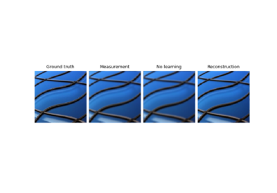
Radio interferometric imaging with deepinverse

Imaging inverse problems with adversarial networks

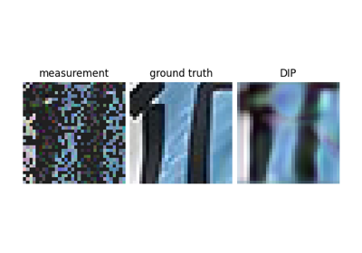
Stacking and concatenating forward operators.

Reconstructing an image using the deep image prior.

Creating your own dataset

Creating a forward operator.

3D diffraction PSF

Training a reconstruction network.

A tour of forward sensing operators

Image deblurring with custom deep explicit prior.

Saving and loading models

A tour of blur operators

Image deblurring with Total-Variation (TV) prior

Image inpainting with wavelet prior

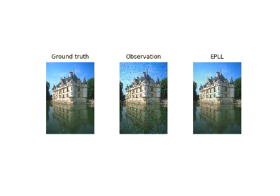
Expected Patch Log Likelihood (EPLL) for Denoising and Inpainting

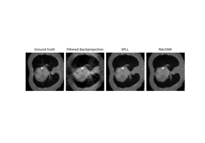
Patch priors for limited-angle computed tomography

Plug-and-Play algorithm with Mirror Descent for Poisson noise inverse problems.

Vanilla PnP for computed tomography (CT).

DPIR method for PnP image deblurring.

Regularization by Denoising (RED) for Super-Resolution.

PnP with custom optimization algorithm (Condat-Vu Primal-Dual)

Uncertainty quantification with PnP-ULA.

Image reconstruction with a diffusion model

Building your custom sampling algorithm.

Implementing DPS

Implementing DiffPIR

Self-supervised learning with measurement splitting

Image transformations for Equivariant Imaging

Self-supervised MRI reconstruction with Artifact2Artifact

Self-supervised denoising with the UNSURE loss.

Self-supervised denoising with the SURE loss.

Self-supervised denoising with the Neighbor2Neighbor loss.

Self-supervised learning with Equivariant Imaging for MRI.

Self-supervised learning from incomplete measurements of multiple operators.

Learned Iterative Soft-Thresholding Algorithm (LISTA) for compressed sensing

Vanilla Unfolded algorithm for super-resolution

Learned iterative custom prior

Deep Equilibrium (DEQ) algorithms for image deblurring

Learned Primal-Dual algorithm for CT scan.

Unfolded Chambolle-Pock for constrained image inpainting

LinearPhysics

Examples using LinearPhysics:

Examples using `LinearPhysics`: