Image deblurring with Total-Variation (TV) prior

This example shows how to use a standard TV prior for image deblurring. The problem writes as \(y = Ax + \epsilon\) where \(A\) is a convolutional operator and \(\epsilon\) is the realization of some Gaussian noise. The goal is to recover the original image \(x\) from the blurred and noisy image \(y\). The TV prior is used to regularize the problem.

import deepinv as dinv
from pathlib import Path
import torch
from torchvision import transforms

from deepinv.optim.data_fidelity import L2
from deepinv.optim.optimizers import optim_builder
from deepinv.utils.demo import load_dataset, load_degradation
from deepinv.utils.plotting import plot, plot_curves

Setup paths for data loading and results.

BASE_DIR = Path(".")
DATA_DIR = BASE_DIR / "measurements"
RESULTS_DIR = BASE_DIR / "results"
DEG_DIR = BASE_DIR / "degradations"

Load base image datasets and degradation operators.

In this example, we use the Set3C dataset and a motion blur kernel from Levin et al. (2009).

# Set the global random seed from pytorch to ensure reproducibility of the example.
torch.manual_seed(0)

device = dinv.utils.get_freer_gpu() if torch.cuda.is_available() else "cpu"

# Set up the variable to fetch dataset and operators.
dataset_name = "set3c"
img_size = 256 if torch.cuda.is_available() else 64
val_transform = transforms.Compose(
    [transforms.CenterCrop(img_size), transforms.ToTensor()]
)

# Generate a motion blur operator.
kernel_index = 1  # which kernel to chose among the 8 motion kernels from 'Levin09.mat'
kernel_torch = load_degradation("Levin09.npy", DEG_DIR / "kernels", index=kernel_index)
kernel_torch = kernel_torch.unsqueeze(0).unsqueeze(
    0
)  # add batch and channel dimensions
dataset = load_dataset(dataset_name, transform=val_transform)

Levin09.npy degradation downloaded in degradations/kernels
Downloading datasets/set3c.zip

  0%|          | 0.00/385k [00:00<?, ?iB/s]
100%|██████████| 385k/385k [00:00<00:00, 15.7MiB/s]
set3c dataset downloaded in datasets

Generate a dataset of blurred images and load it.

We use the BlurFFT class from the physics module to generate a dataset of blurred images.

noise_level_img = 0.05  # Gaussian Noise standard deviation for the degradation
n_channels = 3  # 3 for color images, 1 for gray-scale images
physics = dinv.physics.BlurFFT(
    img_size=(n_channels, img_size, img_size),
    filter=kernel_torch,
    device=device,
    noise_model=dinv.physics.GaussianNoise(sigma=noise_level_img),
)

# Select the first image from the dataset
x = dataset[0][0].unsqueeze(0).to(device)

# Apply the degradation to the image
y = physics(x)

Exploring the total variation prior.

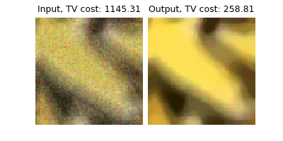
In this example, we will use the total variation prior, which can be done with the deepinv.optim.prior.Prior() class. The prior object represents the cost function of the prior (TV in this case), as well as convenient methods, such as its proximal operator \(\text{prox}_{\tau g}\).

# Set up the total variation prior
prior = dinv.optim.prior.TVPrior(n_it_max=2000)

# Compute the total variation prior cost
cost_tv = prior(y).item()
print(f"Cost TV: g(y) = {cost_tv:.2f}")

# Apply the proximal operator of the TV prior
x_tv = prior.prox(y, gamma=0.1)
cost_tv_prox = prior(x_tv).item()

Cost TV: g(y) = 1145.31

Note

The output of the proximity operator of TV is not the solution to our deblurring problem. It is only a step towards the solution and is used in the proximal gradient descent algorithm to solve the inverse problem.

# Plot the input and the output of the TV proximal operator
imgs = [y, x_tv]
plot(
    imgs,
    titles=[f"Input, TV cost: {cost_tv:.2f}", f"Output, TV cost: {cost_tv_prox:.2f}"],
)

Set up the optimization algorithm to solve the inverse problem.

The problem we want to minimize is the following:

\[\begin{equation*} \underset{x}{\operatorname{min}} \,\, \frac{1}{2} \|Ax-y\|_2^2 + \lambda \|Dx\|_{1,2}(x), \end{equation*}\]

where \(1/2 \|A(x)-y\|_2^2\) is the a data-fidelity term, \(\lambda \|Dx\|_{2,1}(x)\) is the total variation (TV) norm of the image \(x\), and \(\lambda>0\) is a regularisation parameters.

We use a Proximal Gradient Descent (PGD) algorithm to solve the inverse problem.

# Select the data fidelity term
data_fidelity = L2()

# Specify the prior (we redefine it with a smaller number of iteration for faster computation)
prior = dinv.optim.prior.TVPrior(n_it_max=20)

# Logging parameters
verbose = True
plot_convergence_metrics = (
    True  # compute performance and convergence metrics along the algorithm.
)

# Algorithm parameters
stepsize = 1.0
lamb = 1e-2  # TV regularisation parameter
params_algo = {"stepsize": stepsize, "lambda": lamb}
max_iter = 300
early_stop = True

# Instantiate the algorithm class to solve the problem.
model = optim_builder(
    iteration="PGD",
    prior=prior,
    data_fidelity=data_fidelity,
    early_stop=early_stop,
    max_iter=max_iter,
    verbose=verbose,
    params_algo=params_algo,
)

Evaluate the model on the problem and plot the results.

The model returns the output and the metrics computed along the iterations. For computing PSNR, the ground truth image x_gt must be provided.

x_lin = physics.A_adjoint(y)  # linear reconstruction with the adjoint operator

# run the model on the problem.
x_model, metrics = model(
    y, physics, x_gt=x, compute_metrics=True
)  # reconstruction with PGD algorithm

# compute PSNR
print(f"Linear reconstruction PSNR: {dinv.metric.PSNR()(x, x_lin).item():.2f} dB")
print(f"PGD reconstruction PSNR: {dinv.metric.PSNR()(x, x_model).item():.2f} dB")

# plot images. Images are saved in RESULTS_DIR.
imgs = [y, x, x_lin, x_model]
plot(
    imgs,
    titles=["Input", "GT", "Linear", "Recons."],
)

# plot convergence curves
if plot_convergence_metrics:
    plot_curves(metrics)

• 
• 

Linear reconstruction PSNR: 15.01 dB
PGD reconstruction PSNR: 21.43 dB