Learned iterative custom prior

This example shows how to implement a learned unrolled proximal gradient descent algorithm with a custom prior function. The custom prior in use is The algorithm is trained on a dataset of compressed sensing measurements of MNIST images.

from pathlib import Path
import torch
from torchvision import datasets
from torchvision import transforms
import deepinv as dinv
from torch.utils.data import DataLoader
from deepinv.optim.data_fidelity import L2
from deepinv.optim.prior import Prior
from deepinv.optim import PGD
from deepinv.utils import get_data_home

Setup paths for data loading and results.

BASE_DIR = Path(".")
DATA_DIR = BASE_DIR / "measurements"
RESULTS_DIR = BASE_DIR / "results"
CKPT_DIR = BASE_DIR / "ckpts"
ORIGINAL_DATA_DIR = get_data_home()

# Set the global random seed from pytorch to ensure reproducibility of the example.
torch.manual_seed(0)

device = dinv.utils.get_freer_gpu() if torch.cuda.is_available() else "cpu"

Load base image datasets and degradation operators.

In this example, we use MNIST as the base dataset.

img_size = 28
n_channels = 1
operation = "compressed-sensing"
train_dataset_name = "MNIST_train"

# Generate training and evaluation datasets in HDF5 folders and load them.
train_test_transform = transforms.Compose([transforms.ToTensor()])
train_base_dataset = datasets.MNIST(
    root=ORIGINAL_DATA_DIR, train=True, transform=train_test_transform, download=True
)
test_base_dataset = datasets.MNIST(
    root=ORIGINAL_DATA_DIR, train=False, transform=train_test_transform, download=True
)

Generate a dataset of compressed measurements and load it.

We use the compressed sensing class from the physics module to generate a dataset of highly-compressed measurements (10% of the total number of pixels).

The forward operator is defined as \(y = Ax\) where \(A\) is a (normalized) random Gaussian matrix.

# Use parallel dataloader if using a GPU to speed up training, otherwise, as all computes are on CPU, use synchronous
# data loading.
num_workers = 4 if torch.cuda.is_available() else 0

# Generate the compressed sensing measurement operator.
physics = dinv.physics.CompressedSensing(
    m=200, img_size=(n_channels, img_size, img_size), fast=True, device=device
)
my_dataset_name = "demo_LICP"
n_images_max = 200
measurement_dir = DATA_DIR / train_dataset_name / operation
generated_datasets_path = dinv.datasets.generate_dataset(
    train_dataset=train_base_dataset,
    test_dataset=test_base_dataset,
    physics=physics,
    device=device,
    save_dir=measurement_dir,
    train_datapoints=n_images_max,
    test_datapoints=8,
    num_workers=num_workers,
    dataset_filename=str(my_dataset_name),
)

train_dataset = dinv.datasets.HDF5Dataset(path=generated_datasets_path, train=True)
test_dataset = dinv.datasets.HDF5Dataset(path=generated_datasets_path, train=False)

Dataset has been saved at measurements/MNIST_train/compressed-sensing/demo_LICP0.h5

Define the unfolded Proximal Gradient algorithm.

In this example, we propose to minimize a function of the form

\[\min_x \frac{1}{2} \|y - Ax\|_2^2 + \lambda\operatorname{TV}_{\text{smooth}}(x)\]

where \(\operatorname{TV}_{\text{smooth}}\) is a smooth approximation of TV. The proximal gradient iteration (see also deepinv.optim.optim_iterators.PGDIteration) is defined as

\[x_{k+1} = \text{prox}_{\gamma \lambda \operatorname{TV}_{\text{smooth}}}(x_k - \gamma A^T (Ax_k - y))\]

where \(\gamma\) is the stepsize and \(\text{prox}_{g}\) is the proximity operator of \(g(x) =\operatorname{TV}_{\text{smooth}}(x)\).

We first define the prior in a functional form. If the prior is initialized with a list of length max_iter, then a distinct weight is trained for each PGD iteration. For fixed trained model prior across iterations, initialize with a single model.

# Define the image gradient operator
def nabla(I):
    b, c, h, w = I.shape
    G = torch.zeros((b, c, h, w, 2), device=I.device).type(I.dtype)
    G[:, :, :-1, :, 0] = G[:, :, :-1, :, 0] - I[:, :, :-1]
    G[:, :, :-1, :, 0] = G[:, :, :-1, :, 0] + I[:, :, 1:]
    G[:, :, :, :-1, 1] = G[:, :, :, :-1, 1] - I[..., :-1]
    G[:, :, :, :-1, 1] = G[:, :, :, :-1, 1] + I[..., 1:]
    return G


# Define the smooth TV prior as the mse of the image finite difference.
def g(x, *args, **kwargs):
    dx = nabla(x)
    tv_smooth = torch.nn.functional.mse_loss(
        dx, torch.zeros_like(dx), reduction="sum"
    ).sqrt()
    return tv_smooth


# Define the prior. A prior instance from :class:`deepinv.priors` can be simply defined with an explicit potential :math:`g` function as such:
prior = Prior(g=g)

We use deepinv.optim.PGD() with unfold=True to define the unfolded algorithm and set both the stepsizes of the PGD algorithm \(\gamma\) (stepsize) and the soft regularization parameters \(\lambda\) as learnable parameters. These parameters are initialized with a table of length max_iter, yielding a distinct stepsize and lambda value for each iteration of the algorithm. For single stepsize and lambda shared across iterations, initialize with a single float value.

# Unrolled optimization algorithm parameters
max_iter = 10  # Number of unrolled iterations
lambda_reg = [
    1
] * max_iter  # initialization of the regularization parameter. A distinct lamb is trained for each iteration.
stepsize = [
    5
] * max_iter  # initialization of the stepsizes. A distinct stepsize is trained for each iteration.
trainable_params = [
    "stepsize",
    "lambda",
]  # define which parameters are trainable

# Select the data fidelity term
data_fidelity = L2()

# Logging parameters
verbose = True

# Define the unfolded trainable model.
model = PGD(
    unfold=True,
    stepsize=stepsize,
    lambda_reg=lambda_reg,
    trainable_params=trainable_params,
    data_fidelity=data_fidelity,
    max_iter=max_iter,
    prior=prior,
    g_first=True,
)

Define the training parameters.

We now define training-related parameters, number of epochs, optimizer (Adam) and its hyperparameters, and the train and test batch sizes.

# Training parameters
epochs = 5
learning_rate = 0.05  # reduce this parameter when using more epochs

# Choose optimizer and scheduler
optimizer = torch.optim.Adam(model.parameters(), lr=learning_rate)

# Choose supervised training loss
losses = [dinv.loss.SupLoss(metric=torch.nn.L1Loss())]

# Batch sizes and data loaders
train_batch_size = 32
test_batch_size = 32

train_dataloader = DataLoader(
    train_dataset, batch_size=train_batch_size, num_workers=num_workers, shuffle=True
)
test_dataloader = DataLoader(
    test_dataset, batch_size=test_batch_size, num_workers=num_workers, shuffle=False
)

Train the network.

We train the network using the library’s train function.

trainer = dinv.Trainer(
    model,
    physics=physics,
    train_dataloader=train_dataloader,
    eval_dataloader=test_dataloader,
    epochs=epochs,
    device=device,
    losses=losses,
    optimizer=optimizer,
    save_path=str(CKPT_DIR / operation),
    verbose=verbose,
    show_progress_bar=False,  # disable progress bar for better vis in sphinx gallery.
)


model = trainer.train()

The model has 20 trainable parameters
Train epoch 0: TotalLoss=0.123, PSNR=15.523
Eval epoch 0: PSNR=14.9
Best model saved at epoch 1
Train epoch 1: TotalLoss=0.119, PSNR=15.769
Eval epoch 1: PSNR=15.875
Best model saved at epoch 2
Train epoch 2: TotalLoss=0.117, PSNR=15.824
Eval epoch 2: PSNR=16.344
Best model saved at epoch 3
Train epoch 3: TotalLoss=0.118, PSNR=15.838
Eval epoch 3: PSNR=16.324
Train epoch 4: TotalLoss=0.118, PSNR=15.845
Eval epoch 4: PSNR=16.268

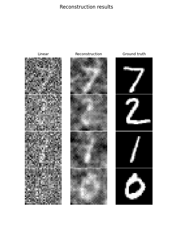
Test the network.

We now test the learned unrolled network on the test dataset. In the plotted results, the first column shows the measurements back-projected in the image domain, the second column shows the output of our network, and the third shows the ground truth.

trainer.test(test_dataloader)

test_sample, _ = next(iter(test_dataloader))
model.eval()
test_sample = test_sample.to(device)

# Get the measurements and the ground truth
y = physics(test_sample)
with torch.no_grad():
    rec = model(y, physics=physics)

backprojected = physics.A_adjoint(y)

dinv.utils.plot(
    [backprojected, rec, test_sample],
    titles=["Linear", "Reconstruction", "Ground truth"],
    suptitle="Reconstruction results",
    save_dir=RESULTS_DIR / "unfolded_pgd" / operation,
)

Eval epoch 0: PSNR=16.268, PSNR no learning=12.072
Test results:
PSNR no learning: 12.072 +- 1.789
PSNR: 16.268 +- 1.325
/home/runner/work/deepinv/deepinv/deepinv/utils/plotting.py:379: UserWarning: This figure was using a layout engine that is incompatible with subplots_adjust and/or tight_layout; not calling subplots_adjust.
  fig.subplots_adjust(top=0.75)

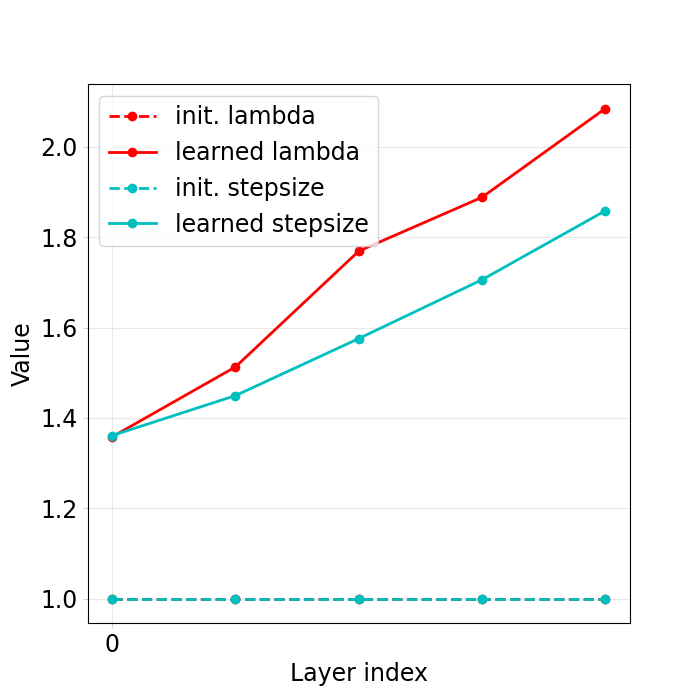
Plotting the weights of the network.

We now plot the weights of the network that were learned and check that they are different from their initialization

dinv.utils.plotting.plot_parameters(
    model,
    init_params={"stepsize": stepsize, "lambda": lambda_reg},
    save_dir=RESULTS_DIR / "unfolded_pgd" / operation,
)