Expected Patch Log Likelihood (EPLL) for Denoising and Inpainting

In this example we use the expected patch log likelihood (EPLL) prior EPLL proposed in “From learning models of natural image patches to whole image restoration”. for denoising and inpainting of natural images. To this end, we consider the inverse problem \(y = Ax+\epsilon\), where \(A\) is either the identity (for denoising) or a masking operator (for inpainting) and \(\epsilon\sim\mathcal{N}(0,\sigma^2 I)\) is white Gaussian noise with standard deviation \(\sigma\).

import torch
from deepinv.optim import EPLL
from deepinv.physics import GaussianNoise, Denoising, Inpainting
from deepinv.loss.metric import PSNR
from deepinv.utils import plot
from deepinv.utils.demo import load_url_image, get_image_url

device = "cuda" if torch.cuda.is_available() else "cpu"

Load test image and model

As default EPLL loads pretrained weights for the Gaussian mixture model which where estimted based on 50 mio patches extracted from the BSDS500 dataset. An example how to estimate the parameters of GMM is included in the demo for limited-angle CT with patch priors.

url = get_image_url("CBSD_0010.png")
test_img = load_url_image(url, grayscale=False).to(device)
patch_size = 6
model = EPLL(channels=test_img.shape[1], patch_size=patch_size, device=device)

Downloading: "https://huggingface.co/deepinv/EPLL/resolve/main/GMM_BSDS_color2.pt?download=true" to /home/runner/.cache/torch/hub/checkpoints/GMM_BSDS_color2.pt

  0%|          | 0.00/35.7M [00:00<?, ?B/s]
  3%|▎         | 1.12M/35.7M [00:00<00:03, 11.7MB/s]
  6%|▋         | 2.25M/35.7M [00:00<00:03, 10.2MB/s]
  9%|▉         | 3.25M/35.7M [00:00<00:03, 10.2MB/s]
 12%|█▏        | 4.25M/35.7M [00:00<00:03, 10.3MB/s]
 15%|█▍        | 5.25M/35.7M [00:00<00:03, 10.3MB/s]
 18%|█▊        | 6.25M/35.7M [00:00<00:02, 10.3MB/s]
 20%|██        | 7.25M/35.7M [00:00<00:02, 10.4MB/s]
 23%|██▎       | 8.25M/35.7M [00:00<00:02, 10.3MB/s]
 26%|██▌       | 9.25M/35.7M [00:00<00:02, 10.3MB/s]
 29%|██▊       | 10.2M/35.7M [00:01<00:02, 10.3MB/s]
 32%|███▏      | 11.2M/35.7M [00:01<00:02, 10.3MB/s]
 34%|███▍      | 12.2M/35.7M [00:01<00:02, 10.3MB/s]
 37%|███▋      | 13.2M/35.7M [00:01<00:02, 10.3MB/s]
 40%|███▉      | 14.2M/35.7M [00:01<00:02, 10.3MB/s]
 43%|████▎     | 15.2M/35.7M [00:01<00:02, 10.4MB/s]
 46%|████▌     | 16.2M/35.7M [00:01<00:01, 10.4MB/s]
 48%|████▊     | 17.2M/35.7M [00:01<00:01, 10.4MB/s]
 51%|█████     | 18.2M/35.7M [00:01<00:01, 10.4MB/s]
 54%|█████▍    | 19.2M/35.7M [00:01<00:01, 10.4MB/s]
 57%|█████▋    | 20.2M/35.7M [00:02<00:01, 10.4MB/s]
 60%|█████▉    | 21.2M/35.7M [00:02<00:01, 10.4MB/s]
 62%|██████▏   | 22.2M/35.7M [00:02<00:01, 10.4MB/s]
 65%|██████▌   | 23.2M/35.7M [00:02<00:01, 10.4MB/s]
 68%|██████▊   | 24.2M/35.7M [00:02<00:01, 10.4MB/s]
 71%|███████   | 25.2M/35.7M [00:02<00:01, 10.4MB/s]
 74%|███████▎  | 26.2M/35.7M [00:02<00:00, 10.4MB/s]
 76%|███████▋  | 27.2M/35.7M [00:02<00:00, 10.4MB/s]
 79%|███████▉  | 28.2M/35.7M [00:02<00:00, 10.4MB/s]
 82%|████████▏ | 29.2M/35.7M [00:02<00:00, 10.4MB/s]
 85%|████████▍ | 30.2M/35.7M [00:03<00:00, 10.4MB/s]
 88%|████████▊ | 31.2M/35.7M [00:03<00:00, 10.4MB/s]
 91%|█████████ | 32.4M/35.7M [00:03<00:00, 10.8MB/s]
 94%|█████████▍| 33.5M/35.7M [00:03<00:00, 10.3MB/s]
 97%|█████████▋| 34.5M/35.7M [00:03<00:00, 10.3MB/s]
100%|█████████▉| 35.6M/35.7M [00:03<00:00, 10.7MB/s]
100%|██████████| 35.7M/35.7M [00:03<00:00, 10.4MB/s]

Denoising

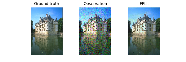
In this setting, the operator \(A\) is the identity; we set the noise level to \(\sigma=25/255\). Define noise model, operator and generate observation

sigma = 0.1
noise_model = GaussianNoise(sigma)
physics = Denoising(device=device, noise_model=noise_model)
observation = physics(test_img)

We use the default choice of the betas in the half quadratic splitting given by \(\beta \in \sigma^{-2} \{1,4,8,16,32\}\). Generally, the betas are hyperparameters, which have to be chosen for each inverse problem separately.

# Reconstruction
with torch.no_grad():
    x_out = model(observation, physics, batch_size=5000)

# PSNR computation and plots.
psnr_obs = PSNR()(observation, test_img).item()
psnr_recon = PSNR()(x_out, test_img).item()

print("PSNRs for Denoising:")
print("Observation: {0:.2f}".format(psnr_obs))
print("EPLL: {0:.2f}".format(psnr_recon))

plot(
    [test_img, observation.clip(0, 1), x_out.clip(0, 1)],
    ["Ground truth", "Observation", "EPLL"],
)

PSNRs for Denoising:
Observation: 20.00
EPLL: 28.96

Inpainting

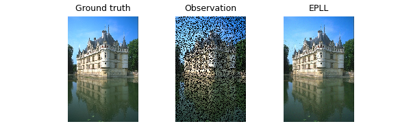
We now turn to a noisy inpainting problem, where the operator \(A\) is a masking operator. Define noise model, operator and generate observation

sigma = 0.01
physics = Inpainting(
    tensor_size=test_img[0].shape,
    mask=0.7,
    device=device,
    noise_model=GaussianNoise(sigma),
)
observation = physics(test_img)

Here, we need a different choice of beta. To this end, we extended the default choice by two values and optimized a constant factor via grid search.

betas = [1.0, 5.0, 10.0, 40.0, 80.0, 160.0, 320.0]

# Reconstruction
with torch.no_grad():
    x_out = model(observation, physics, betas=betas, batch_size=5000)

# PSNR computation and plots
psnr_obs = PSNR()(observation, test_img).item()
psnr_recon = PSNR()(x_out, test_img).item()

print("PSNRs for Inpainting:")
print("Observation: {0:.2f}".format(psnr_obs))
print("EPLL: {0:.2f}".format(psnr_recon))

plot(
    [test_img, observation.clip(0, 1), x_out.clip(0, 1)],
    ["Ground truth", "Observation", "EPLL"],
)

PSNRs for Inpainting:
Observation: 10.94
EPLL: 29.80