PnP with custom optimization algorithm (Primal-Dual Condat-Vu)

This example shows how to define your own optimization algorithm. For example, here, we implement the Primal-Dual Condat-Vu (CV) algorithm, and apply it for Single Pixel Camera reconstruction.

import deepinv as dinv
from pathlib import Path
import torch
from deepinv.models import DnCNN
from deepinv.optim.data_fidelity import L2
from deepinv.optim.prior import PnP
from deepinv.optim.optimizers import BaseOptim
from deepinv.utils import load_example
from deepinv.utils.plotting import plot, plot_curves
from deepinv.optim.optim_iterators import OptimIterator, fStep, gStep

Define a custom optimization algorithm

Creating your optimization algorithm only requires the definition of an iteration step. The iterator should be a subclass of deepinv.optim.OptimIterator.

The Condat-Vu Primal-Dual algorithm is defined as follows:

\[\begin{split}\begin{align*} v_k &= x_k-\tau A^\top z_k \\ x_{k+1} &= \operatorname{prox}_{\tau g}(v_k) \\ u_k &= z_k + \sigma A(2x_{k+1}-x_k) \\ z_{k+1} &= \operatorname{prox}_{\sigma f^*}(u_k) \end{align*}\end{split}\]

where \(f^*\) is the Fenchel-Legendre conjugate of \(f\).

class CVIteration(OptimIterator):
    r"""
    Single iteration of Condat-Vu Primal-Dual.
    """

    def __init__(self, **kwargs):
        super().__init__(**kwargs)
        self.g_step = gStepCV(**kwargs)
        self.f_step = fStepCV(**kwargs)

    def forward(self, X, cur_data_fidelity, cur_prior, cur_params, y, physics):
        r"""
        Single iteration of the Condat-Vu algorithm.

        :param dict X: Dictionary containing the current iterate and the estimated cost.
        :param deepinv.optim.DataFidelity cur_data_fidelity: Instance of the DataFidelity class defining the current data_fidelity.
        :param dict cur_prior: dictionary containing the prior-related term of interest,
            e.g. its proximal operator or gradient.
        :param dict cur_params: dictionary containing the current parameters of the model.
        :param torch.Tensor y: Input data.
        :param deepinv.physics physics: Instance of the physics modeling the data-fidelity term.
        :return: Dictionary `{"est": (x,z), "cost": F}` containing the updated current iterate
            and the estimated current cost.
        """
        x_prev, z_prev = X["est"]
        v = x_prev - cur_params["stepsize"] * physics.A_adjoint(z_prev)
        x = self.g_step(v, cur_prior, cur_params)
        u = z_prev + cur_params["stepsize"] * physics.A(2 * x - x_prev)
        z = self.f_step(u, cur_data_fidelity, cur_params, y, physics)
        F = (
            self.F_fn(x, cur_data_fidelity, cur_params, y, physics)
            if self.has_cost
            and self.F_fn is not None
            and cur_data_fidelity is not None
            and cur_prior is not None
            else None
        )
        return {"est": (x, z), "cost": F}

Define the custom fStep and gStep modules

The iterator relies on custom fStepCV (subclass of deepinv.optim.optim_iterators.fStep) and gStepCV (subclass of deepinv.optim.optim_iterators.gStep) modules.

In this case the fStep module is defined as follows:

\[u_{k+1} = \operatorname{prox}_{\sigma f^*}(u_k)\]

where \(f^*\) is the Fenchel-Legendre conjugate of \(f\). The proximal operator of \(f^*\) is computed using the proximal operator of \(f\) via Moreau’s identity, and the gStep module is a simple proximal step on the prior term \(\lambda g\):

\[x_{k+1} = \operatorname{prox}_{\tau \lambda g}(v_k)\]

class fStepCV(fStep):
    r"""
    Condat-Vu fStep module to compute :math:`\operatorname{prox}_{\sigma f^*}(z_k)``
    """

    def __init__(self, **kwargs):
        super().__init__(**kwargs)

    def forward(self, u, cur_data_fidelity, cur_params, y, phyics):
        r"""
        Single iteration on the data-fidelity term :math:`f`.

        :param torch.Tensor z: Current iterate :math:`z_k = 2Ax_{k+1}-x_k`
        :param deepinv.optim.DataFidelity cur_data_fidelity: Instance of the DataFidelity class defining the current data_fidelity.
        :param dict cur_params: Dictionary containing the current fStep parameters (keys `"stepsize"` and `"lambda"`).
        :param torch.Tensor y: Input data.
        :param deepinv.physics physics: Instance of the physics modeling the data-fidelity term.
        """
        return cur_data_fidelity.d.prox_conjugate(
            u, y, gamma=cur_params["stepsize_dual"]
        )


class gStepCV(gStep):
    r"""
    Condat-Vu gStep module to compute :math:`\operatorname{prox}_{\tau g}(v_k)`
    """

    def __init__(self, **kwargs):
        super().__init__(**kwargs)

    def forward(self, v, cur_prior, cur_params):
        r"""
        Single iteration step on the prior term :math:`\lambda g`.

        :param torch.Tensor x: Current iterate :math:`v_k = x_k-\tau A^\top u_k`.
        :param dict cur_prior: Dictionary containing the current prior.
        :param dict cur_params: Dictionary containing the current gStep parameters
            (keys `"stepsize"` and `"g_param"`).
        """
        return cur_prior.prox(
            v,
            cur_params["g_param"],
            gamma=cur_params["lambda"] * cur_params["stepsize"],
        )

Define the Conva-Vu model as a subclass of deepinv.optim.BaseOptim, in the model of other optimizer of the library, see for example deepinv.optim.ADMM. —————————————————————————————-

class CV(BaseOptim):
    r"""
    Primal-Dual Condat-Vu (CV) optimization algorithm.
    """

    def __init__(
        self,
        data_fidelity=None,
        prior=None,
        lambda_reg=1.0,
        stepsize=1.0,
        stepsize_dual=1.0,
        beta=1.0,
        sigma_denoiser=None,
        **kwargs,
    ):
        params_algo = {
            "lambda": lambda_reg,
            "stepsize": stepsize,
            "stepsize_dual": stepsize_dual,
            "g_param": sigma_denoiser,
            "beta": beta,
        }

        super(CV, self).__init__(
            CVIteration(),
            params_algo=params_algo,
            data_fidelity=data_fidelity,
            prior=prior,
            **kwargs,
        )

Setup paths for data loading and results.

BASE_DIR = Path(".")
RESULTS_DIR = BASE_DIR / "results"

Load base image datasets and degradation operators.

# Set the global random seed from pytorch to ensure reproducibility of the example.
torch.manual_seed(0)

device = dinv.utils.get_freer_gpu() if torch.cuda.is_available() else "cpu"

# Set up the variable to fetch dataset and operators.
method = "PnP"
dataset_name = "set3c"
img_size = 64

x = load_example(
    "barbara.jpeg",
    img_size=img_size,
    grayscale=True,
    resize_mode="resize",
    device=device,
)
operation = "single_pixel"

Set the forward operator

We use the deepinv.physics.SinglePixelCamera class from the physics module to generate a single-pixel measurements. The forward operator consists of the multiplication with the low frequencies of the Hadamard transform.

noise_level_img = 0.03  # Gaussian Noise standard deviation for the degradation
n_channels = 1  # 3 for color images, 1 for gray-scale images
physics = dinv.physics.SinglePixelCamera(
    m=600,
    img_size=(1, 64, 64),
    ordering="cake_cutting",
    noise_model=dinv.physics.GaussianNoise(sigma=noise_level_img),
    device=device,
)

# Use parallel dataloader if using a GPU to speed up training,
# otherwise, as all computes are on CPU, use synchronous data loading.
num_workers = 4 if torch.cuda.is_available() else 0

Set up the PnP algorithm to solve the inverse problem.

We build the PnP model using our custom deepinv.optim.PDCP() function.

The primal dual stepsizes \(\tau\) corresponds to the stepsize key and \(\sigma\) to the sigma key.

For the denoiser, we choose the 1-Lipschitz grayscale DnCNN model (see the pretrained-weights).

# Set up the PnP algorithm parameters :
stepsize = 0.99  # primal stepsize
stepsize_dual = 0.99  # dual stepsize
sigma_denoiser = 0.01  # denoiser parameter (noise level)
max_iter = 200
early_stop = True  # stop the algorithm when convergence is reached

# Select the data fidelity term
data_fidelity = L2()

# Specify the denoising prior
denoiser = DnCNN(
    in_channels=n_channels,
    out_channels=n_channels,
    pretrained="download_lipschitz",
    device=device,
)
prior = PnP(denoiser=denoiser)

# instantiate the algorithm class to solve the IP problem.
model = CV(
    prior=prior,
    data_fidelity=data_fidelity,
    stepsize=stepsize,
    stepsize_dual=stepsize_dual,
    sigma_denoiser=sigma_denoiser,
    early_stop=early_stop,
    max_iter=max_iter,
    verbose=True,
)

Downloading: "https://huggingface.co/deepinv/dncnn/resolve/main/dncnn_sigma2_lipschitz_gray.pth?download=true" to /home/runner/.cache/torch/hub/checkpoints/dncnn_sigma2_lipschitz_gray.pth

  0%|          | 0.00/2.55M [00:00<?, ?B/s]
100%|██████████| 2.55M/2.55M [00:00<00:00, 150MB/s]

Evaluate the model on the problem and plot the results.

The model returns the output and the metrics computed along the iterations. The ground truth image x_gt must be provided for computing the PSNR.

y = physics(x)
x_lin = physics.A_adjoint(y)

# run the model on the problem. For computing the metrics along the iterations, set ``compute_metrics=True``.
x_model, metrics = model(y, physics, x_gt=x, compute_metrics=True)

# compute PSNR
print(f"Linear reconstruction PSNR: {dinv.metric.PSNR()(x, x_lin).item():.2f} dB")
print(f"Model reconstruction PSNR: {dinv.metric.PSNR()(x, x_model).item():.2f} dB")

# plot results
imgs = [x, x_lin, x_model]
plot(imgs, titles=["GT", "Linear", "Recons."], show=True)

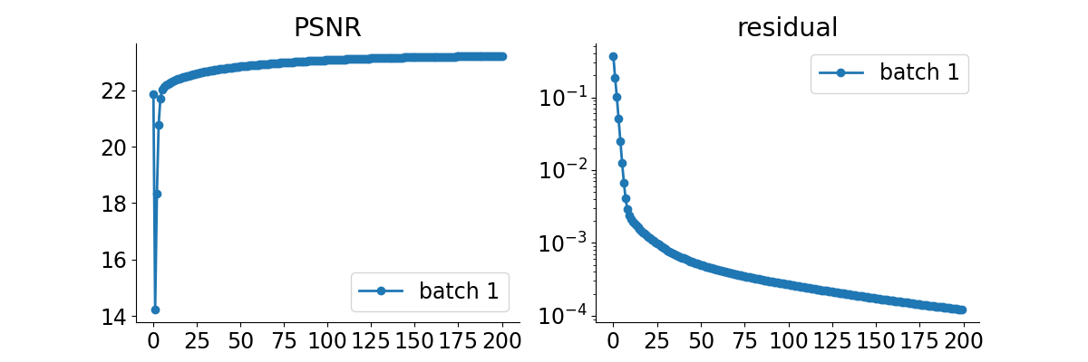
# plot convergence curves
plot_curves(metrics, save_dir=RESULTS_DIR / "curves", show=True)

• 
• 

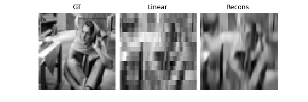
Linear reconstruction PSNR: 23.11 dB
Model reconstruction PSNR: 25.42 dB