DPS – Posterior Sampling with Diffusion Models

In this tutorial, we will go over the steps in the Diffusion Posterior Sampling (DPS) algorithm introduced in Chung et al.[1]. The full algorithm is implemented in deepinv.sampling.DPS.

Let us import the relevant modules and load a sample image of size 64 x 64. This will be used as our ground truth image.

Note

We work with an image of size 64 x 64 to reduce the computational time of this example.

import torch

import deepinv as dinv
from deepinv.utils.plotting import plot
from deepinv.utils import load_example

import matplotlib as mpl

mpl.rcParams["animation.html"] = "jshtml"

device = dinv.utils.get_device()

x_true = load_example("butterfly.png", img_size=64, device=device)
x = x_true.clone()

Selected GPU 0 with 4759.25 MiB free memory

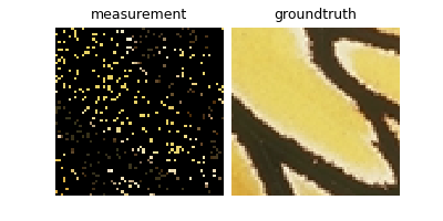
In this tutorial we consider random inpainting as the inverse problem, where the forward operator is implemented in deepinv.physics.Inpainting. In the example that we use, 90% of the pixels will be masked out randomly, and we will additionally have Additive White Gaussian Noise (AWGN) of standard deviation 12.75/255.

sigma = 12.75 / 255.0  # noise level

physics = dinv.physics.Inpainting(
    img_size=(3, x.shape[-2], x.shape[-1]),
    mask=0.1,
    pixelwise=True,
    noise_model=dinv.physics.GaussianNoise(sigma),
    device=device,
)

y = physics(x_true)

plot(
    {
        "Measurement": y,
        "Ground Truth": x_true,
    }
)

Load a pre-trained denoiser

Our DPS implementation relies on a pre-trained denoiser, which is used to approximate the score function of the diffusion process. In this example, we will use a DRUNet denoiser, which is a widely used architecture for image denoising. The example should work with any other denoiser, as long as it takes as input an image and a noise level, and outputs a denoised image.

denoiser = dinv.models.DRUNet(device=device)

The diffusion schedule

Our DPS implementation supports two standard diffusion schedules, which are the deepinv.sampling.VariancePreservingDiffusion (VP) and deepinv.sampling.VarianceExplodingDiffusion (VE) SDEs. In this example, we will use the VP SDE, which is the continuous-time limit of the DDPM sampling process.

DPS approximation

In order to perform gradient-based posterior sampling with diffusion models, we have to be able to compute \(\nabla_{\mathbf{x}_t} \log p(\mathbf{x}_t|\mathbf{y})\). Applying Bayes rule, we have

\[\nabla_{\mathbf{x}_t} \log p(\mathbf{x}_t|\mathbf{y}) = \nabla_{\mathbf{x}_t} \log p(\mathbf{x}_t) + \nabla_{\mathbf{x}_t} \log p(\mathbf{y}|\mathbf{x}_t)\]

For the former term, we can simply plug-in our estimated score function as in Tweedie’s formula. As the latter term is intractable, DPS proposes the following approximation (for details, see Theorem 1 of Chung et al.[1])

\[\nabla_{\mathbf{x}_t} \log p(\mathbf{x}_t|\mathbf{y}) \approx \nabla_{\mathbf{x}_t} \log p(\mathbf{x}_t) + \nabla_{\mathbf{x}_t} \log p(\mathbf{y}|\widehat{\mathbf{x}}_{0}(\mathbf{x_t}))\]

where \(\widehat{\mathbf{x}}_{0}(\mathbf{x_t})\) is the posterior mean of the clean image given the noisy image at time \(t\), which can be estimated with a denoiser network.

Under the assumption of Gaussian noise, the likelihood term can be written as

\[\log p(\mathbf{y}|\widehat{\mathbf{x}}_0(\mathbf{x_t})) = -\frac{\|\mathbf{y} - A\widehat{\mathbf{x}}_0(\mathbf{x_t})\|_2^2}{2\sigma_y^2}.\]

Taking the gradient w.r.t. \(\mathbf{x}_t\) requires backpropagation through the denoiser, which can be easily implemented with PyTorch’s autograd. We provide an implementation of this approximation in deepinv.sampling.DPSDataFidelity, which is a subclass of deepinv.sampling.NoisyDataFidelity.

Note

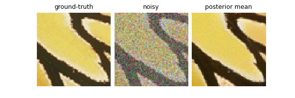
The DPS algorithm assumes that the images are in the range [-1, 1], whereas standard denoisers usually output images in the range [0, 1]. This is why we rescale the images before applying the steps.

from deepinv.sampling import DPSDataFidelity

x0 = x_true * 2.0 - 1.0  # [0, 1] -> [-1, 1]

data_fidelity = DPSDataFidelity(denoiser=denoiser, clip=(-1.0, 1.0))

# choose some arbitrary noise level
sigma_t = 0.2
xt = x0 + sigma_t * torch.randn_like(x0)

# DPS
grad, x0_t = data_fidelity.grad(
    xt / 2 + 0.5, y=y, physics=physics, sigma=sigma_t / 2, get_model_outputs=True
)  # Set get_model_outputs to True to also retrieve the denoised output


# Visualize
plot(
    {
        "Ground Truth": x0,
        "Noisy": xt,
        "Posterior Mean": x0_t,
        "Gradient": grad,
    }
)

DPS Algorithm

As we visited all the key components of DPS, we are now ready to define the algorithm. For every denoising timestep, the algorithm iterates the following

1. Get \(\hat{\mathbf{x}}\) using the denoiser network.

2. Compute \(\nabla_{\mathbf{x}_t} \log p(\mathbf{y}|\hat{\mathbf{x}}_t)\) through backpropagation.

3. Perform reverse diffusion sampling with DDPM(IM), corresponding to an update with \(\nabla_{\mathbf{x}_t} \log p(\mathbf{x}_t)\).

4. Take a gradient step with \(\nabla_{\mathbf{x}_t} \log p(\mathbf{y}|\hat{\mathbf{x}}_t)\).

There are two caveats here. First, in the original work, DPS used DDPM ancestral sampling. As the DDIM sampler Song et al.[2] is a generalization of DDPM in a sense that it retrieves DDPM when \(\alpha = 1.0\). One can freely choose the \(\alpha\) parameter here, it is advisable to keep it \(\alpha = 1.0\) if num_steps=1000. Second, one can also switch to other diffusion schedules, such as the VE SDE, which corresponds to a different noise schedule and sampling process. In this case, the DPS approximation still holds, but the sampling step will be different.

With DeepInverse, we can use the deepinv.sampling.DPS class to perform the above steps with minimal code, with some important parameters:

• weight: corresponds to the \(\lambda\) parameter in the above equation, which controls the strength of the gradient step.

• alpha: corresponds to the stochasticity parameter in the DDIM, which controls the strength of the noise in the reverse diffusion sampling step.

• num_steps: corresponds to the number of denoising steps, which is usually set to 1000 for best performance, but can be reduced to 200 for faster sampling.

Note

For simplicity, we only show the DPS with the VP / VE SDEs, but the algorithm can be easily adapted to arbitrary diffusion processes, for example deepinv.sampling.EDMDiffusionSDE with custom noise schedules. Please refer to the example Building your diffusion posterior sampling method using SDEs for a full demonstration of how to modify the algorithm.

Note

We only use 200 steps to reduce the computational time of this example. As suggested by the authors of DPS, the algorithm works best with num_steps = 1000.

# Instantiate the model
model = dinv.sampling.DPS(
    denoiser=denoiser,
    schedule="vp",
    num_steps=200,
    weight=2.0,
    alpha=0.5,
    verbose=True,
    device=device,
    dtype=torch.float64,
    rng=torch.Generator(device=device),
    minus_one_one=False,
)

# Run the sampling
with torch.no_grad():
    sample, trajectory = model(
        y.clone(),
        physics,
        seed=123,  # for reproducibility!
        get_trajectory=True,
    )
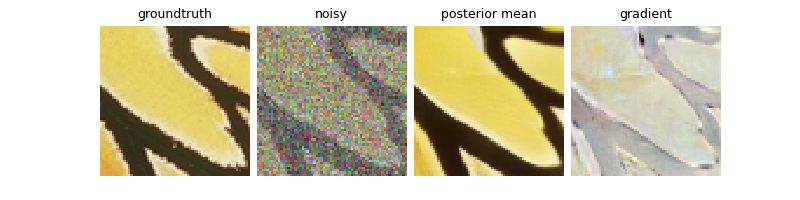
# plot the results
plot(
    {
        "Measurement": y,
        "Model Output": sample,
        "Ground Truth": x_true,
    }
)

anim = dinv.utils.plot_videos(
    trajectory[::10],
    time_dim=0,
    suptitle="DPS Trajectory",
    return_anim=True,
)
anim

  0%|          | 0/199 [00:00<?, ?it/s]
  4%|▎         | 7/199 [00:00<00:03, 61.93it/s]
  7%|▋         | 14/199 [00:00<00:03, 53.76it/s]
 10%|█         | 20/199 [00:00<00:03, 51.67it/s]
 13%|█▎        | 26/199 [00:00<00:03, 50.92it/s]
 16%|█▌        | 32/199 [00:00<00:03, 50.51it/s]
 19%|█▉        | 38/199 [00:00<00:03, 50.42it/s]
 22%|██▏       | 44/199 [00:00<00:03, 49.92it/s]
 25%|██▍       | 49/199 [00:00<00:03, 49.78it/s]
 27%|██▋       | 54/199 [00:01<00:02, 49.76it/s]
 30%|██▉       | 59/199 [00:01<00:02, 49.72it/s]
 32%|███▏      | 64/199 [00:01<00:02, 49.72it/s]
 35%|███▍      | 69/199 [00:01<00:02, 49.53it/s]
 38%|███▊      | 75/199 [00:01<00:02, 49.58it/s]
 40%|████      | 80/199 [00:01<00:02, 49.64it/s]
 43%|████▎     | 85/199 [00:01<00:02, 49.61it/s]
 45%|████▌     | 90/199 [00:01<00:02, 49.58it/s]
 48%|████▊     | 95/199 [00:01<00:02, 49.60it/s]
 51%|█████     | 101/199 [00:02<00:01, 49.97it/s]
 53%|█████▎    | 106/199 [00:02<00:01, 49.69it/s]
 56%|█████▌    | 111/199 [00:02<00:01, 49.56it/s]
 58%|█████▊    | 116/199 [00:02<00:01, 49.39it/s]
 61%|██████    | 121/199 [00:02<00:01, 49.51it/s]
 63%|██████▎   | 126/199 [00:02<00:01, 49.49it/s]
 66%|██████▌   | 131/199 [00:02<00:01, 49.50it/s]
 69%|██████▉   | 137/199 [00:02<00:01, 49.61it/s]
 71%|███████▏  | 142/199 [00:02<00:01, 49.56it/s]
 74%|███████▍  | 147/199 [00:02<00:01, 49.55it/s]
 76%|███████▋  | 152/199 [00:03<00:00, 49.61it/s]
 79%|███████▉  | 158/199 [00:03<00:00, 49.67it/s]
 82%|████████▏ | 163/199 [00:03<00:00, 49.72it/s]
 84%|████████▍ | 168/199 [00:03<00:00, 49.74it/s]
 87%|████████▋ | 173/199 [00:03<00:00, 49.58it/s]
 90%|████████▉ | 179/199 [00:03<00:00, 49.59it/s]
 92%|█████████▏| 184/199 [00:03<00:00, 49.61it/s]
 95%|█████████▌| 190/199 [00:03<00:00, 49.86it/s]
 98%|█████████▊| 195/199 [00:03<00:00, 49.41it/s]
100%|██████████| 199/199 [00:03<00:00, 49.93it/s]
/local/jtachell/deepinv/deepinv/deepinv/utils/plotting.py:408: UserWarning: This figure was using a layout engine that is incompatible with subplots_adjust and/or tight_layout; not calling subplots_adjust.
  fig.subplots_adjust(top=0.75)

Once Loop Reflect

References:

[1] (1,2)

Hyungjin Chung, Jeongsol Kim, Michael Thompson Mccann, Marc Louis Klasky, and Jong Chul Ye. Diffusion posterior sampling for general noisy inverse problems. In The Eleventh International Conference on Learning Representations. 2022.

[2]

Jiaming Song, Chenlin Meng, and Stefano Ermon. Denoising diffusion implicit models. In International Conference on Learning Representations. 2020.