Self-supervised learning from incomplete measurements of multiple operators.

This example shows you how to train a reconstruction network for an inpainting inverse problem on a fully self-supervised way, i.e., using measurement data only.

The dataset consists of pairs \((y_i,A_{g_i})\) where \(y_i\) are the measurements and \(A_{g_i}\) is a binary sampling operator out of \(G\) (i.e., \(g_i\in \{1,\dots,G\}\)).

This self-supervised learning approach is presented in Tachella et al.[1] and minimizes the loss function:

\[\mathcal{L}(\theta) = \sum_{i=1}^{N} \left\|A_{g_i} \hat{x}_{i,\theta} - y_i \right\|_2^2 + \sum_{s=1}^{G} \left\|\hat{x}_{i,\theta} - R_{\theta}(A_s\hat{x}_{i,\theta},A_s) \right\|_2^2\]

where \(R_{\theta}\) is a reconstruction network with parameters \(\theta\), \(y_i\) are the measurements, \(A_s\) is a binary sampling operator, and \(\hat{x}_{i,\theta} = R_{\theta}(y_i,A_{g_i})\).

from pathlib import Path

import torch
from torch.utils.data import DataLoader
from torchvision import datasets, transforms

import deepinv as dinv
from deepinv.utils import get_data_home
from deepinv.models.utils import get_weights_url

Setup paths for data loading and results.

BASE_DIR = Path(".")
DATA_DIR = BASE_DIR / "measurements"
CKPT_DIR = BASE_DIR / "ckpts"
ORIGINAL_DATA_DIR = get_data_home()

# Set the global random seed from pytorch to ensure reproducibility of the example.
torch.manual_seed(0)

device = dinv.utils.get_freer_gpu() if torch.cuda.is_available() else "cpu"

Load base image datasets and degradation operators.

In this example, we use the MNIST dataset for training and testing.

transform = transforms.Compose([transforms.ToTensor()])

train_base_dataset = datasets.MNIST(
    root=ORIGINAL_DATA_DIR, train=True, transform=transform, download=True
)
test_base_dataset = datasets.MNIST(
    root=ORIGINAL_DATA_DIR, train=False, transform=transform, download=True
)

Generate a dataset of subsampled images and load it.

We generate 10 different inpainting operators, each one with a different random mask. If the deepinv.datasets.generate_dataset() receives a list of physics operators, it generates a dataset for each operator and returns a list of paths to the generated datasets.

Note

We only use 10 training images per operator to reduce the computational time of this example. You can use the whole dataset by setting n_images_max = None.

number_of_operators = 10

# defined physics
physics = [
    dinv.physics.Inpainting(mask=0.5, img_size=(1, 28, 28), device=device)
    for _ in range(number_of_operators)
]

# Use parallel dataloader if using a GPU to reduce training time,
# otherwise, as all computes are on CPU, use synchronous data loading.
num_workers = 4 if torch.cuda.is_available() else 0
n_images_max = (
    None if torch.cuda.is_available() else 50
)  # number of images used for training (uses the whole dataset if you have a gpu)

operation = "inpainting"
my_dataset_name = "demo_multioperator_imaging"
measurement_dir = DATA_DIR / "MNIST" / operation
deepinv_datasets_path = dinv.datasets.generate_dataset(
    train_dataset=train_base_dataset,
    test_dataset=test_base_dataset,
    physics=physics,
    device=device,
    save_dir=measurement_dir,
    train_datapoints=n_images_max,
    test_datapoints=10,
    num_workers=num_workers,
    dataset_filename=str(my_dataset_name),
)

train_dataset = [
    dinv.datasets.HDF5Dataset(path=path, train=True) for path in deepinv_datasets_path
]
test_dataset = [
    dinv.datasets.HDF5Dataset(path=path, train=False) for path in deepinv_datasets_path
]

Dataset has been saved at measurements/MNIST/inpainting/demo_multioperator_imaging0.h5
Dataset has been saved at measurements/MNIST/inpainting/demo_multioperator_imaging1.h5
Dataset has been saved at measurements/MNIST/inpainting/demo_multioperator_imaging2.h5
Dataset has been saved at measurements/MNIST/inpainting/demo_multioperator_imaging3.h5
Dataset has been saved at measurements/MNIST/inpainting/demo_multioperator_imaging4.h5
Dataset has been saved at measurements/MNIST/inpainting/demo_multioperator_imaging5.h5
Dataset has been saved at measurements/MNIST/inpainting/demo_multioperator_imaging6.h5
Dataset has been saved at measurements/MNIST/inpainting/demo_multioperator_imaging7.h5
Dataset has been saved at measurements/MNIST/inpainting/demo_multioperator_imaging8.h5
Dataset has been saved at measurements/MNIST/inpainting/demo_multioperator_imaging9.h5

Set up the reconstruction network

As a reconstruction network, we use a simple artifact removal network based on a U-Net. The network is defined as a \(R_{\theta}(y,A)=\phi_{\theta}(A^{\top}y)\) where \(\phi\) is the U-Net.

# Define the unfolded trainable model.
model = dinv.models.ArtifactRemoval(
    backbone_net=dinv.models.UNet(in_channels=1, out_channels=1, scales=3)
)
model = model.to(device)

Set up the training parameters

We choose a self-supervised training scheme with two losses: the measurement consistency loss (MC) and the multi-operator imaging loss (MOI). Necessary and sufficient conditions on the number of operators and measurements are described in Tachella et al.[2].

Note

We use a pretrained model to reduce training time. You can get the same results by training from scratch for 100 epochs.

epochs = 1
learning_rate = 5e-4
batch_size = 64 if torch.cuda.is_available() else 1

# choose self-supervised training losses
# generates 4 random rotations per image in the batch
losses = [dinv.loss.MCLoss(), dinv.loss.MOILoss(physics)]

# choose optimizer and scheduler
optimizer = torch.optim.Adam(model.parameters(), lr=learning_rate, weight_decay=1e-8)
scheduler = torch.optim.lr_scheduler.StepLR(optimizer, step_size=int(epochs * 0.8) + 1)

# start with a pretrained model to reduce training time
file_name = "demo_moi_ckp_10.pth"
url = get_weights_url(model_name="demo", file_name=file_name)
ckpt = torch.hub.load_state_dict_from_url(
    url, map_location=lambda storage, loc: storage, file_name=file_name
)
# load a checkpoint to reduce training time
model.load_state_dict(ckpt["state_dict"])
optimizer.load_state_dict(ckpt["optimizer"])

Downloading: "https://huggingface.co/deepinv/demo/resolve/main/demo_moi_ckp_10.pth?download=true" to /home/runner/.cache/torch/hub/checkpoints/demo_moi_ckp_10.pth

  0%|          | 0.00/23.8M [00:00<?, ?B/s]
100%|██████████| 23.8M/23.8M [00:00<00:00, 545MB/s]

Train the network

To simulate a realistic self-supervised learning scenario, we do not use any supervised metrics for training, such as PSNR or SSIM, which require clean ground truth images.

Tip

We can use the same self-supervised loss for evaluation, as it does not require clean images, to monitor the training process (e.g. for early stopping). This is done automatically when metrics=None and early_stop>0 in the trainer.

verbose = True  # print training information

train_dataloader = [
    DataLoader(dataset, batch_size=batch_size, num_workers=num_workers, shuffle=True)
    for dataset in train_dataset
]
test_dataloader = [
    DataLoader(dataset, batch_size=batch_size, num_workers=num_workers, shuffle=False)
    for dataset in test_dataset
]

# Initialize the trainer
trainer = dinv.Trainer(
    model=model,
    epochs=epochs,
    scheduler=scheduler,
    losses=losses,
    optimizer=optimizer,
    physics=physics,
    device=device,
    train_dataloader=train_dataloader,
    eval_dataloader=test_dataloader,
    metrics=None,  # no supervised metrics
    early_stop=2,  # early stop using the self-supervised loss on the test set
    save_path=str(CKPT_DIR / operation),
    compute_eval_losses=True,  # use self-supervised loss for evaluation
    early_stop_on_losses=True,  # stop using self-supervised eval loss
    verbose=verbose,
    plot_images=True,
    show_progress_bar=False,  # disable progress bar for better vis in sphinx gallery.
    ckp_interval=10,
)

# Train the network
model = trainer.train()

• 
• 

The model has 2069441 trainable parameters
Train epoch 0: MCLoss=0.001, MOILoss=0.001, TotalLoss=0.001
Eval epoch 0: MCLoss=0.0, MOILoss=0.0, TotalLoss=0.001
Best model saved at epoch 1

Test the network

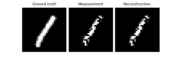
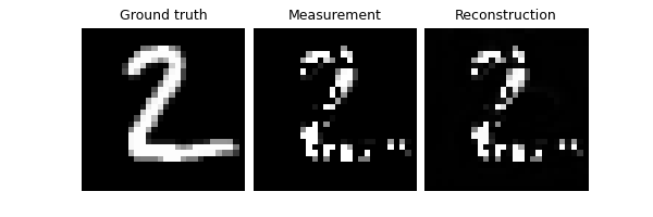
We now assume that we have access to a small test set of ground-truth images to evaluate the performance of the trained network. and we compute the PSNR between the denoised images and the clean ground truth images.

trainer.test(test_dataloader, metrics=dinv.metric.PSNR())

Eval epoch 0: MCLoss=0.0, MOILoss=0.0, TotalLoss=0.001, PSNR=14.829, PSNR no learning=13.689
Test results:
PSNR no learning: 13.689 +- 2.375
PSNR: 14.829 +- 2.368

{'PSNR no learning': 13.689457225799561, 'PSNR no learning_std': 2.3750401284061127, 'PSNR': 14.828871250152588, 'PSNR_std': 2.36779942433444}

References:

[1]

Julián Tachella, Dongdong Chen, and Mike Davies. Unsupervised learning from incomplete measurements for inverse problems. Advances in Neural Information Processing Systems, 35:4983–4995, 2022.

[2]

Julián Tachella, Dongdong Chen, and Mike Davies. Sensing theorems for unsupervised learning in linear inverse problems. Journal of Machine Learning Research, 24(39):1–45, 2023. URL: http://jmlr.org/papers/v24/22-0315.html.