Building your custom sampling algorithm.

This code shows how to build your custom sampling kernel. Here we build a preconditioned Unadjusted Langevin Algorithm (PreconULA) that takes advantage of the singular value decomposition of the forward operator to accelerate the sampling.

import deepinv as dinv
from deepinv.utils.plotting import plot
import torch
from deepinv.sampling import ULA
import numpy as np
from deepinv.utils.demo import load_url_image

Load image from the internet

This example uses an image of Lionel Messi from Wikipedia.

device = dinv.utils.get_freer_gpu() if torch.cuda.is_available() else "cpu"

url = (
    "https://upload.wikimedia.org/wikipedia/commons/b/b4/"
    "Lionel-Messi-Argentina-2022-FIFA-World-Cup_%28cropped%29.jpg"
)
x = load_url_image(url=url, img_size=32).to(device)

Define forward operator and noise model

We use a 5x5 box blur as the forward operator and Gaussian noise as the noise model.

sigma = 0.001  # noise level
physics = dinv.physics.BlurFFT(
    img_size=(3, 32, 32),
    filter=torch.ones((1, 1, 5, 5), device=device) / 25,
    device=device,
    noise_model=dinv.physics.GaussianNoise(sigma=sigma),
)

Generate the measurement

Apply the forward model to generate the noisy measurement.

y = physics(x)

Define the sampling iteration

In order to define a custom sampling kernel (possibly a Markov kernel which depends on the previous sample), we only need to define the iterator which takes the current sample and returns the next sample.

Here we define a preconditioned ULA iterator (for a Gaussian likelihood), which takes into account the singular value decomposition of the forward operator, \(A=USV^{\top}\), in order to accelerate the sampling.

We modify the standard ULA iteration (see deepinv.sampling.ULA) defined as

\[x_{k+1} = x_{k} + \frac{\eta}{\sigma^2} A^{\top}(y-Ax_{k}) + \eta \alpha \nabla \log p(x_{k}) + \sqrt{2\eta}z_{k+1}\]

by using a matrix-valued step size \(\eta = \eta_0 VRV^{\top}\) where \(R\) is a diagonal matrix with entries \(R_{i,i} = \frac{1}{S_{i,i}^2 + \epsilon}\). The parameter \(\epsilon\) is used to avoid numerical issues when \(S_{i,i}^2\) is close to zero. After some algebra, we obtain the following iteration

\[x_{k+1} = x_{k} + \frac{\eta_0}{\sigma^2} V R S (U^{\top}y - S V^{\top}x_{k}) +\eta_0 \alpha V R V^{\top}\nabla \log p(x_{k}) + \sqrt{2\eta_0}V\sqrt{R}z_{k+1}\]

We exploit the methods of deepinv.physics.DecomposablePhysics to compute the matrix-vector products with \(V\) and \(V^{\top}\) efficiently. Note that computing the matrix-vector product with \(R\) and \(S\) is trivial since they are diagonal matrices.

class PULAIterator(torch.nn.Module):
    def __init__(self, step_size, sigma, alpha=1, epsilon=0.01):
        super().__init__()
        self.step_size = step_size
        self.alpha = alpha
        self.noise_std = np.sqrt(2 * step_size)
        self.sigma = sigma
        self.epsilon = epsilon

    def forward(self, x, y, physics, likelihood, prior):
        x_bar = physics.V_adjoint(x)
        y_bar = physics.U_adjoint(y)

        step_size = self.step_size / (self.epsilon + physics.mask.pow(2))

        noise = torch.randn_like(x_bar)
        sigma2_noise = 1 / likelihood.norm
        lhood = -(physics.mask.pow(2) * x_bar - physics.mask * y_bar) / sigma2_noise
        lprior = -physics.V_adjoint(prior.grad(x, self.sigma)) * self.alpha

        return x + physics.V(
            step_size * (lhood + lprior) + (2 * step_size).sqrt() * noise
        )

Build Sampler class

Using our custom iterator, we can build a sampler class by inheriting from the base class deepinv.sampling.MonteCarlo. The base class takes care of the sampling procedure (calculating mean and variance, taking into account sample thinning and burnin iterations, etc), providing a convenient interface to the user.

class PreconULA(dinv.sampling.MonteCarlo):
    def __init__(
        self,
        prior,
        data_fidelity,
        sigma,
        step_size,
        max_iter=1e3,
        thinning=1,
        burnin_ratio=0.1,
        clip=(-1, 2),
        verbose=True,
    ):
        # generate an iterator
        iterator = PULAIterator(step_size=step_size, sigma=sigma)
        # set the params of the base class
        super().__init__(
            iterator,
            prior,
            data_fidelity,
            max_iter=max_iter,
            thinning=thinning,
            burnin_ratio=burnin_ratio,
            clip=clip,
            verbose=verbose,
        )

Define the prior

The score a distribution can be approximated using a plug-and-play denoiser via the deepinv.optim.ScorePrior class.

\[\nabla \log p_{\sigma_d}(x) \approx \frac{1}{\sigma_d^2} \left(D(x) - x\right)\]

This example uses a simple median filter as a plug-and-play denoiser. The hyperparameter \(\sigma_d\) controls the strength of the prior.

prior = dinv.optim.ScorePrior(denoiser=dinv.models.MedianFilter())

Create the preconditioned and standard ULA samplers

We create the preconditioned and standard ULA samplers using the same hyperparameters (step size, number of iterations, etc.).

step_size = 0.5 * (sigma**2)
iterations = int(1e2) if torch.cuda.is_available() else 10
g_param = 0.1

# load Gaussian Likelihood
likelihood = dinv.optim.L2(sigma=sigma)

pula = PreconULA(
    prior=prior,
    data_fidelity=likelihood,
    max_iter=iterations,
    step_size=step_size,
    thinning=1,
    burnin_ratio=0.1,
    verbose=True,
    sigma=g_param,
)


ula = ULA(
    prior=prior,
    data_fidelity=likelihood,
    max_iter=iterations,
    step_size=step_size,
    thinning=1,
    burnin_ratio=0.1,
    verbose=True,
    sigma=g_param,
)

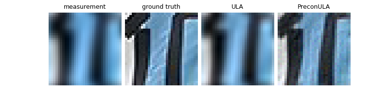
Run sampling algorithms and plot results

Each sampling algorithm returns the posterior mean and variance. We compare the posterior mean of each algorithm with a simple linear reconstruction.

The preconditioned step size of the new sampler provides a significant acceleration to standard ULA, which is evident in the PSNR of the posterior mean.

Note

The preconditioned ULA sampler requires a forward operator with an easy singular value decomposition (e.g. which inherit from deepinv.physics.DecomposablePhysics) and the noise to be Gaussian, whereas ULA is more general.

ula_mean, ula_var = ula(y, physics)

pula_mean, pula_var = pula(y, physics)

# compute linear inverse
x_lin = physics.A_adjoint(y)

# compute PSNR
print(f"Linear reconstruction PSNR: {dinv.utils.metric.cal_psnr(x, x_lin):.2f} dB")
print(f"ULA posterior mean PSNR: {dinv.utils.metric.cal_psnr(x, ula_mean):.2f} dB")
print(
    f"PreconULA posterior mean PSNR: {dinv.utils.metric.cal_psnr(x, pula_mean):.2f} dB"
)

# plot results
imgs = [x_lin, x, ula_mean, pula_mean]
plot(imgs, titles=["measurement", "ground truth", "ULA", "PreconULA"])

  0%|          | 0/10 [00:00<?, ?it/s]
100%|██████████| 10/10 [00:00<00:00, 460.02it/s]
Monte Carlo sampling finished! elapsed time=0.02 seconds

  0%|          | 0/10 [00:00<?, ?it/s]
100%|██████████| 10/10 [00:00<00:00, 407.11it/s]
Monte Carlo sampling finished! elapsed time=0.02 seconds
Linear reconstruction PSNR: 15.48 dB
ULA posterior mean PSNR: 17.30 dB
PreconULA posterior mean PSNR: 22.62 dB