Image transformations for Equivariant Imaging#

This example demonstrates various geometric image transformations implemented in deepinv that can be used in Equivariant Imaging (EI) for self-supervised learning:

Shift: integer pixel 2D shift;
Rotate: 2D image rotation;
Scale: continuous 2D image downscaling;
Euclidean: includes continuous translation, rotation, and reflection, forming the group \(\mathbb{E}(2)\);
Similarity: as above but includes scale, forming the group \(\text{S}(2)\);
Affine: as above but includes shear effects, forming the group \(\text{Aff}(3)\);
Homography: as above but includes perspective (i.e pan and tilt) effects, forming the group \(\text{PGL}(3)\);
PanTiltRotate: pure 3D camera rotation i.e pan, tilt and 2D image rotation.

See docs for full list.

These were proposed in the papers:

Shift, Rotate: Chen et al., Equivariant Imaging: Learning Beyond the Range Space
Scale: Scanvic et al., Self-Supervised Learning for Image Super-Resolution and Deblurring
Homography and the projective geometry framework: Wang et al., Perspective-Equivariant Imaging: an Unsupervised Framework for Multispectral Pansharpening

import torch
from torch.utils.data import DataLoader, random_split
from torchvision.transforms import Compose, ToTensor, CenterCrop, Resize

import deepinv as dinv
from deepinv.utils.demo import get_data_home

device = dinv.utils.get_freer_gpu() if torch.cuda.is_available() else "cpu"

ORIGINAL_DATA_DIR = get_data_home() / "Urban100"

Define transforms. For the transforms that involve 3D camera rotation (i.e pan or tilt), we limit theta_max for display.

transforms = [
    dinv.transform.Shift(),
    dinv.transform.Rotate(),
    dinv.transform.Scale(),
    dinv.transform.Homography(theta_max=10),
    dinv.transform.projective.Euclidean(),
    dinv.transform.projective.Similarity(),
    dinv.transform.projective.Affine(),
    dinv.transform.projective.PanTiltRotate(theta_max=10),
]

Plot transforms on a sample image. Note that, during training, we never have access to these ground truth images x, only partial and noisy measurements y.

x = dinv.utils.load_url_image(dinv.utils.demo.get_image_url("celeba_example.jpg"))
dinv.utils.plot(
    [x] + [t(x) for t in transforms],
    ["Orig"] + [t.__class__.__name__ for t in transforms],
)

Orig, Shift, Rotate, Scale, Homography, Euclidean, Similarity, Affine, PanTiltRotate

Now, we run an inpainting experiment to reconstruct images from images masked with a random mask, without ground truth, using EI. For this example we use the Urban100 images of natural urban scenes. As these scenes are imaged with a camera free to move and rotate in the world, all of the above transformations are valid invariances that we can impose on the unknown image set \(x\in X\).

dataset = dinv.datasets.Urban100HR(
    root=ORIGINAL_DATA_DIR,
    download=True,
    transform=Compose([ToTensor(), Resize(256), CenterCrop(256)]),
)

train_dataset, test_dataset = random_split(dataset, (0.8, 0.2))

train_dataloader = DataLoader(train_dataset, shuffle=True)
test_dataloader = DataLoader(test_dataset)

# Use physics to generate data online
physics = dinv.physics.Inpainting((3, 256, 256), mask=0.6, device=device)

  0%|          | 0/135388067 [00:00<?, ?it/s]
  0%|          | 192k/129M [00:00<01:17, 1.74MB/s]
  1%|          | 1.00M/129M [00:00<00:24, 5.50MB/s]
  4%|▍         | 5.06M/129M [00:00<00:05, 21.9MB/s]
 11%|█▏        | 14.6M/129M [00:00<00:02, 51.9MB/s]
 19%|█▉        | 24.5M/129M [00:00<00:01, 70.5MB/s]
 24%|██▍       | 31.3M/129M [00:00<00:01, 67.4MB/s]
 30%|███       | 39.2M/129M [00:00<00:01, 72.3MB/s]
 38%|███▊      | 48.9M/129M [00:00<00:01, 81.1MB/s]
 45%|████▌     | 58.1M/129M [00:00<00:00, 85.9MB/s]
 53%|█████▎    | 68.0M/129M [00:01<00:00, 91.2MB/s]
 60%|█████▉    | 77.3M/129M [00:01<00:00, 93.1MB/s]
 67%|██████▋   | 87.0M/129M [00:01<00:00, 95.7MB/s]
 75%|███████▌  | 96.9M/129M [00:01<00:00, 97.9MB/s]
 82%|████████▏ | 106M/129M [00:01<00:00, 97.8MB/s]
 90%|████████▉ | 116M/129M [00:01<00:00, 95.1MB/s]
 97%|█████████▋| 126M/129M [00:01<00:00, 97.7MB/s]
100%|██████████| 129M/129M [00:01<00:00, 80.6MB/s]

Extracting:   0%|          | 0/101 [00:00<?, ?it/s]
Extracting:  19%|█▉        | 19/101 [00:00<00:00, 186.16it/s]
Extracting:  40%|███▉      | 40/101 [00:00<00:00, 197.91it/s]
Extracting:  61%|██████▏   | 62/101 [00:00<00:00, 207.87it/s]
Extracting:  82%|████████▏ | 83/101 [00:00<00:00, 196.91it/s]
Extracting: 100%|██████████| 101/101 [00:00<00:00, 195.28it/s]
Dataset has been successfully downloaded.

For training, use a small UNet, Adam optimizer, EI loss with homography transform, and the deepinv.Trainer functionality:

Note

We only train for a single epoch in the demo, but it is recommended to train multiple epochs in practice.

model = dinv.models.UNet(
    in_channels=3, out_channels=3, scales=2, circular_padding=True, batch_norm=False
).to(device)

losses = [
    dinv.loss.MCLoss(),
    dinv.loss.EILoss(dinv.transform.Homography(theta_max=10, device=device)),
]

optimizer = torch.optim.Adam(model.parameters(), lr=1e-3, weight_decay=1e-8)

model = dinv.Trainer(
    model=model,
    physics=physics,
    online_measurements=True,
    train_dataloader=train_dataloader,
    eval_dataloader=test_dataloader,
    epochs=1,
    losses=losses,
    optimizer=optimizer,
    verbose=True,
    show_progress_bar=False,
    save_path=None,
    device=device,
).train()

The model has 444867 trainable parameters
Train epoch 0: MCLoss=0.008, TotalLoss=0.02, EILoss=0.024, PSNR=9.754
Eval epoch 0: PSNR=17.21
Best model saved at epoch 1

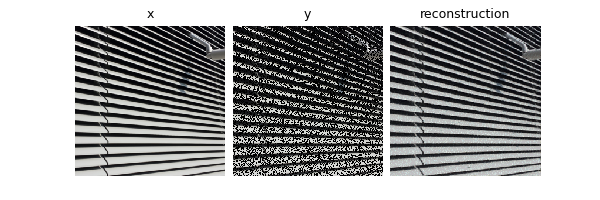
Show results of a pretrained model trained using a larger UNet for 40 epochs:

model = dinv.models.UNet(
    in_channels=3, out_channels=3, scales=3, circular_padding=True, batch_norm=False
).to(device)

ckpt = torch.hub.load_state_dict_from_url(
    dinv.models.utils.get_weights_url("ei", "Urban100_inpainting_homography_model.pth"),
    map_location=device,
)

model.load_state_dict(ckpt["state_dict"])

x = next(iter(train_dataloader))
x = x.to(device)
y = physics(x)
x_hat = model(y)

dinv.utils.plot([x, y, x_hat], ["x", "y", "reconstruction"])

Downloading: "https://huggingface.co/deepinv/ei/resolve/main/Urban100_inpainting_homography_model.pth?download=true" to /home/runner/.cache/torch/hub/checkpoints/Urban100_inpainting_homography_model.pth

  0%|          | 0.00/7.90M [00:00<?, ?B/s]
 81%|████████  | 6.38M/7.90M [00:00<00:00, 42.5MB/s]
100%|██████████| 7.90M/7.90M [00:00<00:00, 49.4MB/s]

Total running time of the script: (2 minutes 12.865 seconds)

Gallery generated by Sphinx-Gallery

Image transformations for Equivariant Imaging#

This Page