Reconstructing an image using the deep image prior.

This code shows how to reconstruct a noisy and incomplete image using the deep image prior.

This method is based on the paper “Deep Image Prior” by Ulyanov et al. (2018), and reconstructs an image by minimizing the loss function

\[\min_{\theta} \|y-Af_{\theta}(z)\|^2\]

where \(z\) is a random input and \(f_{\theta}\) is a convolutional decoder network with parameters \(\theta\). The minimization should be stopped early to avoid overfitting. The method uses the Adam optimizer.

import deepinv as dinv
from deepinv.utils.plotting import plot
import torch
from deepinv.utils import load_url_image

Load image from the internet

This example uses an image of Lionel Messi from Wikipedia.

device = dinv.utils.get_freer_gpu() if torch.cuda.is_available() else "cpu"

url = (
    "https://upload.wikimedia.org/wikipedia/commons/b/b4/"
    "Lionel-Messi-Argentina-2022-FIFA-World-Cup_%28cropped%29.jpg"
)
x = load_url_image(url=url, img_size=32).to(device)

# Set the global random seed from pytorch to ensure reproducibility of the example.
torch.manual_seed(0)

<torch._C.Generator object at 0x7f35cb7091f0>

Define forward operator and noise model

We use image inpainting as the forward operator and Gaussian noise as the noise model.

sigma = 0.1  # noise level
physics = dinv.physics.Inpainting(mask=0.5, tensor_size=x.shape[1:], device=device)
physics.noise_model = dinv.physics.GaussianNoise(sigma=sigma)

Generate the measurement

We apply the forward model to generate the noisy measurement.

y = physics(x)

Define the deep image prior

This method only works with certain convolutional decoder networks. We recommend using the network deepinv.models.ConvDecoder.

Note

The number of iterations and learning rate have been set manually to obtain good results. However, these values may not be optimal for all problems. We recommend experimenting with different values.

Note

Here we run a small number of iterations to reduce the runtime of the example. However, the results could be improved by running more iterations.

iterations = 100
lr = 1e-2  # learning rate for the optimizer.
channels = 64  # number of channels per layer in the decoder.
in_size = [2, 2]  # size of the input to the decoder.
backbone = dinv.models.ConvDecoder(
    img_shape=x.shape[1:], in_size=in_size, channels=channels
).to(device)

f = dinv.models.DeepImagePrior(
    backbone,
    learning_rate=lr,
    iterations=iterations,
    verbose=True,
    input_size=[channels] + in_size,
).to(device)

Run DIP algorithm and plot results

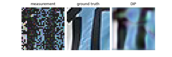
We run the DIP algorithm and plot the results.

The good performance of DIP is somewhat surprising, since the network has many parameters and could potentially overfit the noisy measurement data. However, the architecture acts as an implicit regularizer, providing good reconstructions if the optimization is stopped early. While this phenomenon is not yet well understood, there has been some efforts to explain it. For example, see “The Neural Tangent Link Between CNN Denoisers and Non-Local Filters”.

dip = f(y, physics)

# compute linear inverse
x_lin = physics.A_adjoint(y)

# compute PSNR
print(f"Linear reconstruction PSNR: {dinv.metric.PSNR()(x, x_lin).item():.2f} dB")
print(f"DIP PSNR: {dinv.metric.PSNR()(x, dip).item():.2f} dB")

# plot results
plot([x_lin, x, dip], titles=["measurement", "ground truth", "DIP"])

  0%|          | 0/100 [00:00<?, ?it/s]
 11%|█         | 11/100 [00:00<00:00, 105.31it/s]
 23%|██▎       | 23/100 [00:00<00:00, 110.43it/s]
 35%|███▌      | 35/100 [00:00<00:00, 112.16it/s]
 47%|████▋     | 47/100 [00:00<00:00, 112.92it/s]
 59%|█████▉    | 59/100 [00:00<00:00, 113.34it/s]
 71%|███████   | 71/100 [00:00<00:00, 113.63it/s]
 83%|████████▎ | 83/100 [00:00<00:00, 113.81it/s]
 95%|█████████▌| 95/100 [00:00<00:00, 114.02it/s]
100%|██████████| 100/100 [00:00<00:00, 113.12it/s]
Linear reconstruction PSNR: 8.80 dB
DIP PSNR: 19.24 dB