Uncertainty quantification with PnP-ULA.

This code shows you how to use sampling algorithms to quantify uncertainty of a reconstruction from incomplete and noisy measurements.

ULA obtains samples by running the following iteration:

\[x_{k+1} = x_k + \alpha \eta \nabla \log p_{\sigma}(x_k) + \eta \nabla \log p(y|x_k) + \sqrt{2 \eta} z_k\]

where \(z_k \sim \mathcal{N}(0, I)\) is a Gaussian random variable, \(\eta\) is the step size and \(\alpha\) is a parameter controlling the regularization.

The PnP-ULA method is described in the paper Laumont et al.[1].

import deepinv as dinv
from deepinv.utils.plotting import plot
import torch
from deepinv.utils import load_example

Load image from the internet

This example uses an image of Messi.

device = dinv.utils.get_device()

x = load_example("messi.jpg", img_size=32).to(device)

Selected GPU 0 with 1991.125 MiB free memory

Define forward operator and noise model

This example uses inpainting as the forward operator and Gaussian noise as the noise model.

sigma = 0.1  # noise level
physics = dinv.physics.Inpainting(mask=0.5, img_size=x.shape[1:], device=device)
physics.noise_model = dinv.physics.GaussianNoise(sigma=sigma)

# Set the global random seed from pytorch to ensure reproducibility of the example.
torch.manual_seed(0)

<torch._C.Generator object at 0x7f3bc1553b70>

Define the likelihood

Since the noise model is Gaussian, the negative log-likelihood is the L2 loss.

\[-\log p(y|x) \propto \frac{1}{2\sigma^2} \|y-Ax\|^2\]

# load Gaussian Likelihood
likelihood = dinv.optim.data_fidelity.L2(sigma=sigma)

Define the prior

The score a distribution can be approximated using Tweedie’s formula via the deepinv.optim.ScorePrior class.

\[\nabla \log p_{\sigma}(x) \approx \frac{1}{\sigma^2} \left(D(x,\sigma)-x\right)\]

This example uses a pretrained DnCNN model. From a Bayesian point of view, the score plays the role of the gradient of the negative log prior The hyperparameter sigma_denoiser (\(sigma\)) controls the strength of the prior.

In this example, we use a pretrained DnCNN model using the deepinv.loss.FNEJacobianSpectralNorm loss, which makes sure that the denoiser is firmly non-expansive (see Terris et al.[2]), and helps to stabilize the sampling algorithm.

sigma_denoiser = 2 / 255
prior = dinv.optim.ScorePrior(
    denoiser=dinv.models.DnCNN(pretrained="download_lipschitz")
).to(device)

Create the MCMC sampler

Here we use the Unadjusted Langevin Algorithm (ULA) to sample from the posterior defined in deepinv.sampling.ULAIterator. The hyperparameter step_size controls the step size of the MCMC sampler, regularization controls the strength of the prior and iterations controls the number of iterations of the sampler.

regularization = 0.9
step_size = 0.01 * (sigma**2)
iterations = int(5e3) if torch.cuda.is_available() else 10
params = {
    "step_size": step_size,
    "alpha": regularization,
    "sigma": sigma_denoiser,
}
f = dinv.sampling.sampling_builder(
    "ULA",
    prior=prior,
    data_fidelity=likelihood,
    max_iter=iterations,
    params_algo=params,
    thinning=1,
    verbose=True,
)

Generate the measurement

We apply the forward model to generate the noisy measurement.

y = physics(x)

Run sampling algorithm and plot results

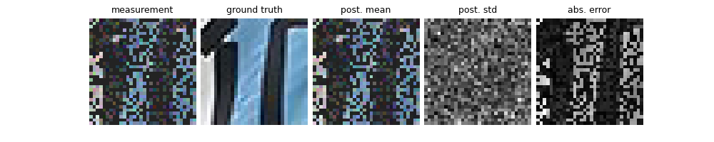
The sampling algorithm returns the posterior mean and variance. We compare the posterior mean with a simple linear reconstruction.

mean, var = f.sample(y, physics)

# compute linear inverse
x_lin = physics.A_adjoint(y)

# compute PSNR
print(f"Linear reconstruction PSNR: {dinv.metric.PSNR()(x, x_lin).item():.2f} dB")
print(f"Posterior mean PSNR: {dinv.metric.PSNR()(x, mean).item():.2f} dB")

# plot results
error = (mean - x).abs().sum(dim=1).unsqueeze(1)  # per pixel average abs. error
std = var.sum(dim=1).unsqueeze(1).sqrt()  # per pixel average standard dev.
imgs = [x_lin, x, mean, std / std.flatten().max(), error / error.flatten().max()]
plot(
    imgs,
    titles=["measurement", "ground truth", "post. mean", "post. std", "abs. error"],
)

  0%|          | 0/5000 [00:00<?, ?it/s]
  2%|▏         | 87/5000 [00:00<00:05, 862.74it/s]
  4%|▍         | 188/5000 [00:00<00:05, 944.60it/s]
  6%|▌         | 292/5000 [00:00<00:04, 985.50it/s]
  8%|▊         | 396/5000 [00:00<00:04, 1003.91it/s]
 10%|█         | 500/5000 [00:00<00:04, 1013.76it/s]
 12%|█▏        | 604/5000 [00:00<00:04, 1020.76it/s]
 14%|█▍        | 707/5000 [00:00<00:04, 1002.06it/s]
 16%|█▌        | 811/5000 [00:00<00:04, 1012.26it/s]
 18%|█▊        | 915/5000 [00:00<00:04, 1018.76it/s]
 20%|██        | 1018/5000 [00:01<00:03, 1020.25it/s]
 22%|██▏       | 1121/5000 [00:01<00:03, 1006.58it/s]
 24%|██▍       | 1222/5000 [00:01<00:03, 999.19it/s]
 26%|██▋       | 1322/5000 [00:01<00:03, 994.47it/s]
 28%|██▊       | 1422/5000 [00:01<00:03, 991.26it/s]
 30%|███       | 1522/5000 [00:01<00:03, 989.27it/s]
 32%|███▏      | 1621/5000 [00:01<00:03, 987.44it/s]
 34%|███▍      | 1720/5000 [00:01<00:03, 979.19it/s]
 36%|███▋      | 1819/5000 [00:01<00:03, 980.34it/s]
 38%|███▊      | 1918/5000 [00:01<00:03, 981.17it/s]
 40%|████      | 2017/5000 [00:02<00:03, 975.91it/s]
 42%|████▏     | 2116/5000 [00:02<00:02, 978.40it/s]
 44%|████▍     | 2215/5000 [00:02<00:02, 979.52it/s]
 46%|████▋     | 2314/5000 [00:02<00:02, 980.50it/s]
 48%|████▊     | 2413/5000 [00:02<00:02, 979.42it/s]
 50%|█████     | 2512/5000 [00:02<00:02, 979.70it/s]
 52%|█████▏    | 2611/5000 [00:02<00:02, 980.11it/s]
 54%|█████▍    | 2710/5000 [00:02<00:02, 980.74it/s]
 56%|█████▌    | 2809/5000 [00:02<00:02, 981.57it/s]
 58%|█████▊    | 2908/5000 [00:02<00:02, 981.69it/s]
 60%|██████    | 3007/5000 [00:03<00:02, 982.37it/s]
 62%|██████▏   | 3106/5000 [00:03<00:01, 982.75it/s]
 64%|██████▍   | 3205/5000 [00:03<00:01, 983.14it/s]
 66%|██████▌   | 3304/5000 [00:03<00:01, 983.35it/s]
 68%|██████▊   | 3403/5000 [00:03<00:01, 983.27it/s]
 70%|███████   | 3502/5000 [00:03<00:01, 977.12it/s]
 72%|███████▏  | 3601/5000 [00:03<00:01, 979.53it/s]
 74%|███████▍  | 3699/5000 [00:03<00:01, 974.10it/s]
 76%|███████▌  | 3798/5000 [00:03<00:01, 977.44it/s]
 78%|███████▊  | 3897/5000 [00:03<00:01, 979.51it/s]
 80%|███████▉  | 3995/5000 [00:04<00:01, 975.55it/s]
 82%|████████▏ | 4093/5000 [00:04<00:00, 975.98it/s]
 84%|████████▍ | 4191/5000 [00:04<00:00, 977.01it/s]
 86%|████████▌ | 4290/5000 [00:04<00:00, 979.31it/s]
 88%|████████▊ | 4389/5000 [00:04<00:00, 980.05it/s]
 90%|████████▉ | 4488/5000 [00:04<00:00, 980.92it/s]
 92%|█████████▏| 4587/5000 [00:04<00:00, 980.54it/s]
 94%|█████████▎| 4686/5000 [00:04<00:00, 981.53it/s]
 96%|█████████▌| 4785/5000 [00:04<00:00, 982.22it/s]
 98%|█████████▊| 4884/5000 [00:04<00:00, 982.79it/s]
100%|█████████▉| 4983/5000 [00:05<00:00, 982.82it/s]
100%|██████████| 5000/5000 [00:05<00:00, 984.75it/s]
Iteration 4999, current converge crit. = 1.43E-05, objective = 1.00E-03
Iteration 4999, current converge crit. = 3.42E-04, objective = 1.00E-03
Linear reconstruction PSNR: 8.55 dB
Posterior mean PSNR: 22.31 dB

References:

[1]

Rémi Laumont, Valentin De Bortoli, Andrés Almansa, Julie Delon, Alain Durmus, and Marcelo Pereyra. Bayesian imaging using plug & play priors: when langevin meets tweedie. SIAM Journal on Imaging Sciences, 15(2):701–737, 2022.

[2]

Matthieu Terris, Audrey Repetti, Jean-Christophe Pesquet, and Yves Wiaux. Building firmly nonexpansive convolutional neural networks. In ICASSP 2020-2020 IEEE International Conference on Acoustics, Speech and Signal Processing (ICASSP), 8658–8662. IEEE, 2020.