Remote sensing with satellite images

In this example we demonstrate remote sensing inverse problems for multispectral satellite imaging.

These have important applications for image restoration in environmental monitoring, urban planning, disaster recovery etc.

We will demonstrate pan-sharpening, i.e., recovering high-resolution multispectral images from measurement pairs of low-resolution multispectral images and high-resolution panchromatic (single-band) images with the forward operator deepinv.physics.Pansharpen.

We will also demonstrate other inverse problems including compressive spectral imaging and hyperspectral unmixing.

We provide a convenient satellite image dataset for pan-sharpening deepinv.datasets.NBUDataset provided in the paper A Large-Scale Benchmark Data Set for Evaluating Pansharpening Performance which includes data from several satellites such as WorldView satellites.

Tip

For remote sensing experiments, DeepInverse provides the following classes:

• Pan-sharpening

• Compressive spectral imaging

• Hyperspectral unmixing

• Super resolution

• Satellite imagery dataset

• Metrics for multispectral data: QNR, SpectralAngleMapper, ERGAS

import deepinv as dinv
import torch

Load raw pan-sharpening measurements

The dataset includes raw pansharpening measurements containing (MS, PAN) where MS are the low-res (4-band) multispectral and PAN are the high-res panchromatic images. Note there are no ground truth images!

Note

The pan-sharpening measurements are provided as a deepinv.utils.TensorList, since the pan-sharpening physics deepinv.physics.Pansharpen is a stacked physics combining deepinv.physics.Downsampling and deepinv.physics.Decolorize. See the User Guide Combining Physics for more information.

Note, for plotting purposes we only plot the first 3 bands (RGB).

Note also that the linear adjoint must assume the unknown spectral response function (SRF).

DATA_DIR = dinv.utils.get_data_home()
dataset = dinv.datasets.NBUDataset(DATA_DIR, return_pan=True, download=True)

y = dataset[0].unsqueeze(0)  # MS (1,4,256,256), PAN (1,1,1024,1024)

physics = dinv.physics.Pansharpen((4, 1024, 1024), factor=4)

# Pansharpen with classical Brovey method
x_hat = physics.A_dagger(y)  # shape (1,4,1024,1024)

dinv.utils.plot(
    [
        y[0][:, :3],
        y[1],  # Note this will be interpolated to match high-res image size
        x_hat[:, :3],
        physics.A_adjoint(y)[:, :3],
    ],
    titles=[
        "Input MS",
        "Input PAN",
        "Pseudo-inverse using Brovey method",
        "Linear adjoint",
    ],
    dpi=1200,
)

Downloading datasets/nbu/gaofen-1.zip

  0%|          | 0/7914941 [00:00<?, ?it/s]
 16%|█▌        | 1.19M/7.55M [00:00<00:00, 10.9MB/s]
 30%|██▉       | 2.25M/7.55M [00:00<00:00, 11.0MB/s]
 44%|████▍     | 3.31M/7.55M [00:00<00:00, 10.9MB/s]
 58%|█████▊    | 4.38M/7.55M [00:00<00:00, 10.9MB/s]
 72%|███████▏  | 5.44M/7.55M [00:00<00:00, 10.1MB/s]
 85%|████████▌ | 6.44M/7.55M [00:00<00:00, 10.1MB/s]
100%|██████████| 7.55M/7.55M [00:00<00:00, 10.6MB/s]
100%|██████████| 7.55M/7.55M [00:00<00:00, 10.6MB/s]

Extracting:   0%|          | 0/12 [00:00<?, ?it/s]
Extracting: 100%|██████████| 12/12 [00:00<00:00, 889.64it/s]
Dataset has been successfully downloaded.

Evaluate performance - note we can only use QNR as we have no GT

qnr = dinv.metric.QNR()
print(qnr(x_net=x_hat, x=None, y=y, physics=physics))

tensor([0.4133])

Simulate remote-sensing measurements

We can also simulate measurements from various remote sensing inverse problems so that we have pairs of measurements and ground truth. Now, the dataset loads ground truth images x:

dataset = dinv.datasets.NBUDataset(DATA_DIR, return_pan=False)

x = dataset[0].unsqueeze(0)  # just MS of shape 1,4,256,256

For compressive spectral imaging, we use the coded-aperture snapshot spectral imaging (CASSI) model, which is a popular hyperspectral imaging method. See deepinv.physics.CompressiveSpectralImaging

physics = dinv.physics.CompressiveSpectralImaging(x.shape[1:], mode="sd")
y = physics(x)  # 1,1,256,256
dinv.utils.plot([x[:, :3], y], titles=["Image x", "CASSI meas. y"])

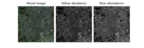
For hyperspectral unmixing, our images are the measurements and we seek to recover abundances given the endmember matrix in the linear mixing model. In this toy example, we perform unmixing with 2 endmembers: one purely yellow and one purely blue.

physics = dinv.physics.HyperSpectralUnmixing(
    M=torch.tensor([[0.5, 0.5, 0.0, 0.0], [0.0, 0.0, 1.0, 0.0]])
)
abundance = physics.A_adjoint(x)  # 1,2,256,256
dinv.utils.plot(
    [x[:, :3], abundance[:, [0]], abundance[:, [1]]],
    titles=["Mixed image", "Yellow abudance", "Blue abundance"],
)

For the pansharpening physics, we assume a flat spectral response function, but this can also be jointly learned. We simulate Gaussian noise on the panchromatic images.

physics = dinv.physics.Pansharpen((4, 256, 256), factor=4, srf="flat")

y = physics(x)

# Pansharpen with classical Brovey method
x_hat = physics.A_dagger(y)

Solving pan-sharpening with neural networks

The pan-sharpening physics is compatible with the rest of the DeepInverse library so we can solve the inverse problem using any method provided in the library. For example, we use here the PanNet model.

This model can be trained using losses such as supervised learning using deepinv.loss.SupLoss or self-supervised learning using Equivariant Imaging deepinv.loss.EILoss, which was applied to pan-sharpening in Wang et al., Perspective-Equivariant Imaging: an Unsupervised Framework for Multispectral Pansharpening

For evaluation, we use the standard full-reference metrics (ERGAS, SAM) and no-reference (QNR).

Note

This is a tiny example using 5 images. We demonstrate training for 1 epoch for speed, but you can train from scratch using 50 epochs.

model = dinv.models.PanNet(hrms_shape=(4, 256, 256))
x_net = model(y, physics)

Example training loss using measurement consistency on the multispectral images and Stein’s Unbiased Risk Estimate on the panchromatic images. For metrics, we use standard full-reference and no-reference multispectral pan-sharpening metrics, since ground-truth is now available.

loss = dinv.loss.StackedPhysicsLoss(
    [dinv.loss.MCLoss(), dinv.loss.SureGaussianLoss(0.05)]
)

sam = dinv.metric.distortion.SpectralAngleMapper()
ergas = dinv.metric.distortion.ERGAS(factor=4)
qnr = dinv.metric.QNR()
print(sam(x_hat, x), ergas(x_hat, x), qnr(x_hat, x=None, y=y, physics=physics))

tensor([0.0545]) tensor([4.1428]) tensor([0.4736])

For training, we first load optimizer and pretrained model, then train using the deepinv Trainer.

optimizer = torch.optim.Adam(model.parameters())

from deepinv.models.utils import get_weights_url

file_name = "demo_nbu_pansharpen.pth"
url = get_weights_url(model_name="demo", file_name=file_name)
ckpt = torch.hub.load_state_dict_from_url(
    url, map_location=lambda storage, loc: storage, file_name=file_name
)
model.load_state_dict(ckpt["state_dict"])
optimizer.load_state_dict(ckpt["optimizer"])

from torch.utils.data import DataLoader

trainer = dinv.Trainer(
    model=model,
    physics=physics,
    optimizer=optimizer,
    losses=loss,
    metrics=[sam, ergas],
    train_dataloader=DataLoader(dataset),
    epochs=1,
    online_measurements=True,
    plot_images=False,
    compare_no_learning=True,
    no_learning_method="A_dagger",
    show_progress_bar=False,
)

trainer.train()
trainer.test(DataLoader(dataset))

Downloading: "https://huggingface.co/deepinv/demo/resolve/main/demo_nbu_pansharpen.pth?download=true" to /home/runner/.cache/torch/hub/checkpoints/demo_nbu_pansharpen.pth

  0%|          | 0.00/955k [00:00<?, ?B/s]
100%|██████████| 955k/955k [00:00<00:00, 12.0MB/s]
The model has 77124 trainable parameters
Train epoch 0: TotalLoss=0.002, SpectralAngleMapper=0.28, ERGAS=23.228
Eval epoch 0: SpectralAngleMapper=0.275, SpectralAngleMapper no learning=0.039, ERGAS=24.077, ERGAS no learning=4.343
Test results:
SpectralAngleMapper no learning: 0.039 +- 0.011
SpectralAngleMapper: 0.275 +- 0.009
ERGAS no learning: 4.343 +- 1.165
ERGAS: 24.077 +- 9.450

{'SpectralAngleMapper no learning': np.float64(0.03942249119281769), 'SpectralAngleMapper no learning_std': np.float64(0.011435804285508791), 'SpectralAngleMapper': np.float64(0.27505362033843994), 'SpectralAngleMapper_std': np.float64(0.008716236651714974), 'ERGAS no learning': np.float64(4.343320846557617), 'ERGAS no learning_std': np.float64(1.1653334600767409), 'ERGAS': np.float64(24.07730712890625), 'ERGAS_std': np.float64(9.449944205275518)}

Plot sample results:

dinv.utils.plot(
    [
        x[:, :3],
        y[0][:, :3],
        y[1],
        x_hat[:, :3],
        x_net[:, :3],
    ],
    titles=["x HRMS", "y LRMS", "y PAN", "Estimate (classical)", "Estimate (PanNet)"],
)