Single photon lidar operator for depth ranging.

In this example we show how to use the deepinv.physics.SinglePhotonLidar forward model.

import deepinv as dinv
import torch
import matplotlib.pyplot as plt

# Use matplotlib config from deepinv to get nice plots
from deepinv.utils.plotting import config_matplotlib

config_matplotlib()

Create forward model

We create a lidar model with 100 bins per pixel and a Gaussian impulse response function with a standard deviation of 2 bins.

The forward model for the case of a single depth per pixel is defined as (e.g. see this paper):

\[y_{i,j,t} = \mathcal{P}(h(t-d_{i,j}) r_{i,j} + b_{i,j})\]

where \(\mathcal{P}\) is the Poisson noise model, \(h(t)\) is a Gaussian impulse response function at time \(t\), \(d_{i,j}\) is the depth of the scene at pixel \((i,j)\), \(r_{i,j}\) is the intensity of the scene at pixel \((i,j)\) and \(b_{i,j}\) is the background noise at pixel \((i,j)\).

device = dinv.utils.get_freer_gpu() if torch.cuda.is_available() else "cpu"
bins = 100
irf_sigma = 2
physics = dinv.physics.SinglePhotonLidar(bins=bins, sigma=irf_sigma, device=device)

Generate toy signal and measurement

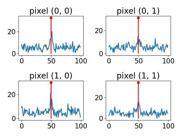
We generate a toy signal with a single peak per pixel located around the 50th bin and a signal-to-background ratio of 10%.

Signals should have size (B, 3, H, W) where the first channel contains the depth of the scene, the second channel contains the intensity of the scene and the third channel contains the per pixel background noise levels.

The measurement associated with a signal has size (B, bins, H, W).

sbr = 0.1
signal = 50
bkg_level = signal / sbr / bins
depth = bins / 2

# depth
d = torch.ones(1, 1, 2, 2, device=device) * depth
# signal
r = torch.ones_like(d) * signal
# background
b = torch.ones_like(d) * bkg_level

x = torch.cat([d, r, b], dim=1)  # signal of size (B, 3, H, W)

y = physics(x)  # measurement of size (B, bins, H, W)

Apply matched filtering to recover the signal and plot the results

We apply matched filtering to recover the signal and plot the results.

The measurements are shown in blue and the depth and intensity of the recovered signals are shown in red.

xhat = physics.A_dagger(y)

plt.figure()
for i in range(2):
    for j in range(2):
        plt.subplot(2, 2, i * 2 + j + 1)
        plt.plot(y[0, :, i, j].detach().cpu().numpy())
        plt.stem(
            xhat[0, 0, i, j].detach().cpu().numpy(),
            xhat[0, 1, i, j].detach().cpu().numpy() / 4,
            linefmt="red",
            markerfmt="red",
        )
        plt.title(f"pixel ({i}, {j})")


plt.tight_layout()
plt.show()

/home/runner/work/deepinv/deepinv/deepinv/physics/lidar.py:78: UserWarning: Using padding='same' with even kernel lengths and odd dilation may require a zero-padded copy of the input be created (Triggered internally at ../aten/src/ATen/native/Convolution.cpp:1036.)
  x = torch.nn.functional.conv1d(y, self.irf, padding="same")