
Note
Go to the end to download the full example code.
Random phase retrieval and reconstruction methods.#
This example shows how to create a random phase retrieval operator and generate phaseless measurements from a given image. The example showcases 4 different reconstruction methods to recover the image from the phaseless measurements:
Gradient descent with random initialization;
Spectral methods;
Gradient descent with spectral methods initialization;
Gradient descent with PnP denoisers.
General setup#
import deepinv as dinv
from pathlib import Path
import torch
import matplotlib.pyplot as plt
from deepinv.models import DRUNet
from deepinv.optim.data_fidelity import L2
from deepinv.optim.prior import PnP, Zero
from deepinv.optim.optimizers import optim_builder
from deepinv.utils.demo import load_example
from deepinv.utils.plotting import plot
from deepinv.optim.phase_retrieval import (
    correct_global_phase,
    cosine_similarity,
)
from deepinv.models.complex import to_complex_denoiser

BASE_DIR = Path(".")
RESULTS_DIR = BASE_DIR / "results"
# Set global random seed to ensure reproducibility.
torch.manual_seed(0)

device = dinv.utils.get_freer_gpu() if torch.cuda.is_available() else "cpu"
Load image from the internet#
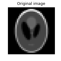
We use the standard test image “Shepp–Logan phantom”.
tensor(0.) tensor(0.7412)
Visualization#
We use the customized plot() function in deepinv to visualize the original image.
Signal construction#
We use the original image as the phase information for the complex signal. The original value range is [0, 1], and we map it to the phase range [-pi/2, pi/2].
x_phase = torch.exp(1j * x * torch.pi - 0.5j * torch.pi)

# Every element of the signal should have unit norm.
assert torch.allclose(x_phase.real**2 + x_phase.imag**2, torch.tensor(1.0))
Measurements generation#
Create a random phase retrieval operator with an oversampling ratio (measurements/pixels) of 5.0, and generate measurements from the signal with additive Gaussian noise.
# Define physics information
oversampling_ratio = 5.0
img_size = x.shape[1:]
m = int(oversampling_ratio * torch.prod(torch.tensor(img_size)))
n_channels = 1  # 3 for color images, 1 for gray-scale images

# Create the physics
physics = dinv.physics.RandomPhaseRetrieval(
    m=m,
    img_size=img_size,
    device=device,
)

# Generate measurements
y = physics(x_phase)
Reconstruction with gradient descent and random initialization#
First, we use the function deepinv.optim.L2 as the data fidelity function, and the class deepinv.optim.optim_iterators.GDIteration as the optimizer to run a gradient descent algorithm. The initial guess is a random complex signal.
data_fidelity = L2()
prior = Zero()
iterator = dinv.optim.optim_iterators.GDIteration()
# Parameters for the optimizer, including stepsize and regularization coefficient.
optim_params = {"stepsize": 0.06, "lambda": 1.0, "g_param": []}
num_iter = 1000

# Initial guess
x_phase_gd_rand = torch.randn_like(x_phase)

loss_hist = []

for _ in range(num_iter):
    res = iterator(
        {"est": (x_phase_gd_rand,), "cost": 0},
        cur_data_fidelity=data_fidelity,
        cur_prior=prior,
        cur_params=optim_params,
        y=y,
        physics=physics,
    )
    x_phase_gd_rand = res["est"][0]
    loss_hist.append(data_fidelity(x_phase_gd_rand, y, physics).cpu())

print("initial loss:", loss_hist[0])
print("final loss:", loss_hist[-1])
# Plot the loss curve
plt.plot(loss_hist)
plt.yscale("log")
plt.title("loss curve (gradient descent with random initialization)")
plt.show()
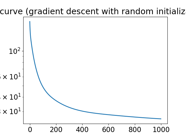
initial loss: tensor([190.4569])
final loss: tensor([28.0710])
Phase correction and signal reconstruction#
The solution of the optimization algorithm x_est may be any phase-shifted version of the original complex signal x_phase, i.e., x_est = a * x_phase where a is an arbitrary unit norm complex number.
Therefore, we use the function deepinv.optim.phase_retrieval.correct_global_phase to correct the global phase shift of the estimated signal x_est to make it closer to the original signal x_phase.
We then use torch.angle to extract the phase information. With the range of the returned value being [-pi/2, pi/2], we further normalize it to be [0, 1].
This operation will later be done for all the reconstruction methods.
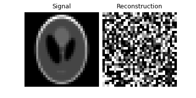
# correct possible global phase shifts
x_gd_rand = correct_global_phase(x_phase_gd_rand, x_phase)
# extract phase information and normalize to the range [0, 1]
x_gd_rand = torch.angle(x_gd_rand) / torch.pi + 0.5

plot([x, x_gd_rand], titles=["Signal", "Reconstruction"], rescale_mode="clip")
Reconstruction with spectral methods#
Spectral methods deepinv.optim.phase_retrieval.spectral_methods offers a good initial guess on the original signal. Moreover, deepinv.physics.RandomPhaseRetrieval uses spectral methods as its default reconstruction method A_dagger, which we can directly call.
# Spectral methods return a tensor with unit norm.
x_phase_spec = physics.A_dagger(y, n_iter=300)
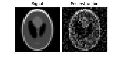
Phase correction and signal reconstruction#
# correct possible global phase shifts
x_spec = correct_global_phase(x_phase_spec, x_phase)
# extract phase information and normalize to the range [0, 1]
x_spec = torch.angle(x_spec) / torch.pi + 0.5
plot([x, x_spec], titles=["Signal", "Reconstruction"], rescale_mode="clip")
Reconstruction with gradient descent and spectral methods initialization#
The estimate from spectral methods can be directly used as the initial guess for the gradient descent algorithm.
# Initial guess from spectral methods
x_phase_gd_spec = physics.A_dagger(y, n_iter=300)

loss_hist = []
for _ in range(num_iter):
    res = iterator(
        {"est": (x_phase_gd_spec,), "cost": 0},
        cur_data_fidelity=data_fidelity,
        cur_prior=prior,
        cur_params=optim_params,
        y=y,
        physics=physics,
    )
    x_phase_gd_spec = res["est"][0]
    loss_hist.append(data_fidelity(x_phase_gd_spec, y, physics).cpu())

print("intial loss:", loss_hist[0])
print("final loss:", loss_hist[-1])
plt.plot(loss_hist)
plt.yscale("log")
plt.title("loss curve (gradient descent with spectral initialization)")
plt.show()
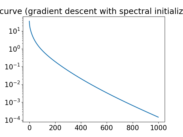
intial loss: tensor([42.0413])
final loss: tensor([0.0034])
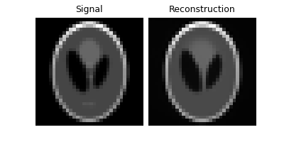
Phase correction and signal reconstruction#
# correct possible global phase shifts
x_gd_spec = correct_global_phase(x_phase_gd_spec, x_phase)
# extract phase information and normalize to the range [0, 1]
x_gd_spec = torch.angle(x_gd_spec) / torch.pi + 0.5
plot([x, x_gd_spec], titles=["Signal", "Reconstruction"], rescale_mode="clip")

Reconstruction with gradient descent and PnP denoisers#
We can also use the Plug-and-Play (PnP) framework to incorporate denoisers as regularizers in the optimization algorithm. We use a deep denoiser as the prior, which is trained on a large dataset of natural images.
# Load the pre-trained denoiser
denoiser = DRUNet(
    in_channels=n_channels,
    out_channels=n_channels,
    pretrained="download",  # automatically downloads the pretrained weights, set to a path to use custom weights.
    device=device,
)
# The original denoiser is designed for real-valued images, so we need to convert it to a complex-valued denoiser for phase retrieval problems.
denoiser_complex = to_complex_denoiser(denoiser, mode="abs_angle")

# Algorithm parameters
data_fidelity = L2()
prior = PnP(denoiser=denoiser_complex)
params_algo = {"stepsize": 0.30, "g_param": 0.04}
max_iter = 100
early_stop = True
verbose = True

# Instantiate the algorithm class to solve the IP problem.
model = optim_builder(
    iteration="PGD",
    prior=prior,
    data_fidelity=data_fidelity,
    early_stop=early_stop,
    max_iter=max_iter,
    verbose=verbose,
    params_algo=params_algo,
)

# Run the algorithm
x_phase_pnp, metrics = model(y, physics, x_gt=x_phase, compute_metrics=True)
Downloading: "https://huggingface.co/deepinv/drunet/resolve/main/drunet_deepinv_gray_finetune_26k.pth?download=true" to /home/runner/.cache/torch/hub/checkpoints/drunet_deepinv_gray_finetune_26k.pth

  0%|          | 0.00/125M [00:00<?, ?B/s]
  9%|▉         | 11.2M/125M [00:00<00:01, 118MB/s]
 19%|█▉        | 24.2M/125M [00:00<00:00, 128MB/s]
 45%|████▍     | 55.5M/125M [00:00<00:00, 219MB/s]
 68%|██████▊   | 84.4M/125M [00:00<00:00, 251MB/s]
 92%|█████████▏| 115M/125M [00:00<00:00, 276MB/s]
100%|██████████| 125M/125M [00:00<00:00, 246MB/s]
Phase correction and signal reconstruction#
# correct possible global phase shifts
x_pnp = correct_global_phase(x_phase_pnp, x_phase)
# extract phase information and normalize to the range [0, 1]
x_pnp = torch.angle(x_pnp) / (2 * torch.pi) + 0.5
plot([x, x_pnp], titles=["Signal", "Reconstruction"], rescale_mode="clip")
Overall comparison#
We visualize the original image and the reconstructed images from the four methods. We further compute the PSNR (Peak Signal-to-Noise Ratio) scores (higher better) for every reconstruction and their cosine similarities with the original image (range in [0,1], higher better). In conclusion, gradient descent with random intialization provides a poor reconstruction, while spectral methods provide a good initial estimate which can later be improved by gradient descent to acquire the best reconstruction results. Besides, the PnP framework with a deep denoiser as the prior also provides a very good denoising results as it exploits prior information about the set of natural images.
imgs = [x, x_gd_rand, x_spec, x_gd_spec, x_pnp]
plot(
    imgs,
    titles=["Original", "GD random", "Spectral", "GD spectral", "PnP"],
    save_dir=RESULTS_DIR / "images",
    show=True,
    rescale_mode="clip",
)

# Compute metrics
print(
    f"GD Random reconstruction, PSNR: {dinv.metric.cal_psnr(x, x_gd_rand).item():.2f} dB; cosine similarity: {cosine_similarity(x_phase_gd_rand, x_phase).item():.3f}."
)
print(
    f"Spectral reconstruction, PSNR: {dinv.metric.cal_psnr(x, x_spec).item():.2f} dB; cosine similarity: {cosine_similarity(x_phase_spec, x_phase).item():.3f}."
)
print(
    f"GD Spectral reconstruction, PSNR: {dinv.metric.cal_psnr(x, x_gd_spec).item():.2f} dB; cosine similarity: {cosine_similarity(x_phase_gd_spec, x_phase).item():.3f}."
)
print(
    f"PnP reconstruction, PSNR: {dinv.metric.cal_psnr(x, x_pnp).item():.2f} dB; cosine similarity: {cosine_similarity(x_phase_pnp, x_phase).item():.3f}."
)
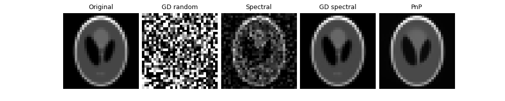
GD Random reconstruction, PSNR: 3.95 dB; cosine similarity: 0.201.
Spectral reconstruction, PSNR: 18.88 dB; cosine similarity: 0.902.
GD Spectral reconstruction, PSNR: 50.80 dB; cosine similarity: 1.000.
PnP reconstruction, PSNR: 13.83 dB; cosine similarity: 0.999.
Total running time of the script: (0 minutes 33.930 seconds)