Plug-and-Play algorithm with Mirror Descent for Poisson noise inverse problems.

This is a simple example to show how to use a mirror descent algorithm for solving an inverse problem with Poisson noise.

The Mirror descent with RED denoiser writes

\[x_{k+1} = \nabla \phi ( \nabla \phi^*(x_k) - \tau \nabla \distance{A(x_k)}{y} - \tau ( x_k - D_\sigma(x)))\]

where \(\phi\) is a convex Bergman potential, \(\distance{A(x)}{y}\) is the data fidelity term and \(D_\sigma(x)\) is a denoiser.

In this example, we use the DnCNN denoiser. As the observation has been corrupted with Poisson noise, we use the deepinv.optim.PoissonLikelihood data-fidelity term. In https://publications.ut-capitole.fr/id/eprint/25852/1/25852.pdf, it is shown that, with this data-fidelity term, the right Bregman potential to use is Burg’s entropy deepinv.optim.bregman.BurgEntropy.

import deepinv as dinv
from pathlib import Path
import torch
from torch.utils.data import DataLoader
from deepinv.optim.data_fidelity import PoissonLikelihood
from deepinv.optim.prior import RED
from deepinv.optim import optim_builder
from deepinv.optim.bregman import BurgEntropy
from deepinv.utils.demo import load_url_image, get_image_url
from deepinv.utils.plotting import plot, plot_curves

Setup paths for data loading and results.

BASE_DIR = Path(".")
ORIGINAL_DATA_DIR = BASE_DIR / "datasets"
DATA_DIR = BASE_DIR / "measurements"
RESULTS_DIR = BASE_DIR / "results"
CKPT_DIR = BASE_DIR / "ckpts"

# Set the global random seed from pytorch to ensure reproducibility of the example.
torch.manual_seed(0)

img_size = 64
device = dinv.utils.get_freer_gpu() if torch.cuda.is_available() else "cpu"
url = get_image_url("butterfly.png")
x_true = load_url_image(url=url, img_size=img_size).to(device)
x = x_true.clone()


n_channels = 3  # 3 for color images, 1 for gray-scale images
operation = "deblurring"

# Degradation parameters
noise_level_img = 1 / 40  # Poisson Noise gain

# Generate the gaussian blur operator with Poisson noise.
physics = dinv.physics.BlurFFT(
    img_size=(n_channels, img_size, img_size),
    filter=dinv.physics.blur.gaussian_blur(),
    device=device,
    noise_model=dinv.physics.PoissonNoise(gain=noise_level_img),
)

Define the PnP algorithm.

The chosen algorithm is here MD (Mirror Descent).

# Select the data fidelity term, here Poisson likelihood due to the use of Poisson noise in the forward operator.
data_fidelity = PoissonLikelihood(gain=noise_level_img)

# Set up the denoising prior. Note that we use a Gaussian noise denoiser, even if the observation noise is Poisson.
prior = RED(denoiser=dinv.models.DnCNN(depth=20, pretrained="download").to(device))

# Set up the optimization parameters
max_iter = 200  # number of iterations
stepsize = 1.0  # stepsize of the algorithm
sigma_denoiser = 0.05  # noise level parameter of the Gaussian denoiser
params_algo = {  # wrap all the restoration parameters in a 'params_algo' dictionary. In particular, this is here that we define the bregman potential used in the mirror descent algorithm.
    "stepsize": stepsize,
    "g_param": sigma_denoiser,
}

# Logging parameters
verbose = True

# Define the unfolded trainable model.
model = optim_builder(
    iteration="MD",
    prior=prior,
    data_fidelity=data_fidelity,
    early_stop=True,
    max_iter=max_iter,
    verbose=verbose,
    params_algo=params_algo,
    bregman_potential=BurgEntropy(),
)

Evaluate the model on the problem and plot the results.

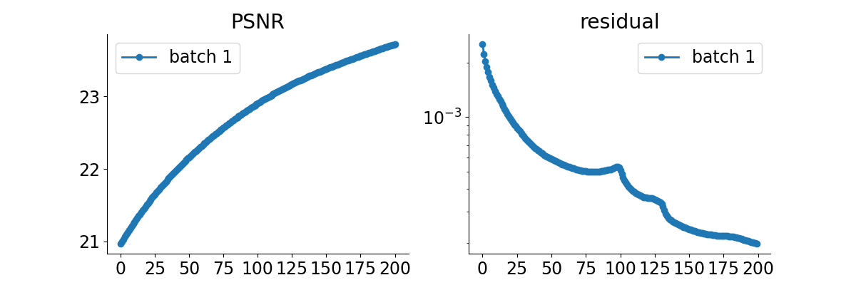
The model returns the output and the metrics computed along the iterations. For computing PSNR, the ground truth image x_gt must be provided.

y = physics(x)
x_lin = physics.A_adjoint(y)

# run the model on the problem.
with torch.no_grad():
    x_model, metrics = model(
        y, physics, x_gt=x, compute_metrics=True
    )  # reconstruction with PnP algorithm

# compute PSNR
print(f"Linear reconstruction PSNR: {dinv.metric.PSNR()(x, x_lin).item():.2f} dB")
print(f"PnP reconstruction PSNR: {dinv.metric.PSNR()(x, x_model).item():.2f} dB")

# plot images. Images are saved in RESULTS_DIR.
imgs = [y, x, x_lin, x_model]
plot(
    imgs,
    titles=["Input", "GT", "Linear", "Recons."],
    save_dir=RESULTS_DIR / "images",
    show=True,
)

# plot convergence curves. Metrics are saved in RESULTS_DIR.
plot_curves(metrics, save_dir=RESULTS_DIR / "curves", show=True)

• 
• 

Linear reconstruction PSNR: 20.97 dB
PnP reconstruction PSNR: 23.72 dB