Note
Go to the end to download the full example code.
Tour of MRI functionality in DeepInverse#
This example presents the various datasets, forward physics and models available in DeepInverse for Magnetic Resonance Imaging (MRI) problems:
Physics:
deepinv.physics.MRI,deepinv.physics.MultiCoilMRI,deepinv.physics.DynamicMRIDatasets: raw kspace with the FastMRI dataset
deepinv.datasets.FastMRISliceDatasetand an in-memory easy-to-use versiondeepinv.datasets.SimpleFastMRISliceDataset, and raw dynamic k-t-space data with the CMRxRecon dataset.Models:
deepinv.models.VarNet(VarNet Hammernik et al.[1], E2E-VarNet Sriram et al.[2]),deepinv.models.MoDL(a simple MoDL Aggarwal et al.[3] unrolled model)
Contents:
Get started with FastMRI (singlecoil + multicoil)
Train an accelerated MRI with neural networks
Load raw FastMRI data (singlecoil + multicoil)
Train using raw data
Explore 3D MRI
Explore dynamic MRI
import deepinv as dinv
import torch, torchvision
from torch.utils.data import DataLoader

device = dinv.utils.get_freer_gpu() if torch.cuda.is_available() else "cpu"
rng = torch.Generator(device=device).manual_seed(0)
1. Get started with FastMRI#
You can get started with our simple FastMRI mini slice subsets which provide quick, easy-to-use, in-memory datasets which can be used for simulation experiments.
Important
By using this dataset, you confirm that you have agreed to and signed the FastMRI data use agreement.
See also
- Datasets
deepinv.datasets.FastMRISliceDatasetdeepinv.datasets.SimpleFastMRISliceDataset We provide convenient datasets to easily load both raw and reconstructed FastMRI images. You can download more data on the FastMRI site.
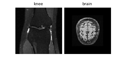
Load mini demo knee and brain datasets (original data is 320x320 but we resize to 128 for speed):
transform = torchvision.transforms.Resize(128)
knee_dataset = dinv.datasets.SimpleFastMRISliceDataset(
    dinv.utils.get_data_home(),
    anatomy="knee",
    transform=transform,
    train=True,
    download=True,
)
brain_dataset = dinv.datasets.SimpleFastMRISliceDataset(
    dinv.utils.get_data_home(),
    anatomy="brain",
    transform=transform,
    train=True,
    download=True,
)

img_size = knee_dataset[0].shape[-2:]  # (128, 128)
dinv.utils.plot({"knee": knee_dataset[0], "brain": brain_dataset[0]})
  0%|          | 0/820529 [00:00<?, ?it/s]
100%|██████████| 801k/801k [00:00<00:00, 78.9MB/s]

  0%|          | 0/820534 [00:00<?, ?it/s]
100%|██████████| 801k/801k [00:00<00:00, 84.4MB/s]
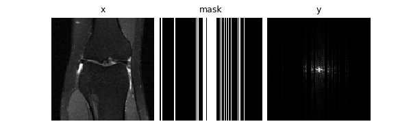
Let’s start with single-coil MRI. We can define a constant Cartesian 4x
undersampling mask by sampling once from a physics generator. The mask,
data and measurements will all be of shape (B, C, H, W) where
C=2 is the real and imaginary parts.
physics_generator = dinv.physics.generator.GaussianMaskGenerator(
    img_size=img_size, acceleration=4, rng=rng, device=device
)
mask = physics_generator.step()["mask"]

physics = dinv.physics.MRI(mask=mask, img_size=img_size, device=device)

dinv.utils.plot(
    {
        "x": (x := next(iter(DataLoader(knee_dataset)))),
        "mask": mask,
        "y": physics(x).clamp(-1, 1),
    }
)
print("Shapes:", x.shape, physics.mask.shape)
Shapes: torch.Size([1, 2, 128, 128]) torch.Size([1, 2, 128, 128])
We can next generate an accelerated single-coil MRI measurement dataset. Let’s use knees for training and brains for testing.
We can also use the physics generator to randomly sample a new mask per sample, and save the masks alongside the measurements.
Note that you could alternatively train using online_measurements, where you can generate
random measurements on the fly.
dataset_path = dinv.datasets.generate_dataset(
    train_dataset=knee_dataset,
    test_dataset=brain_dataset,
    val_dataset=None,
    physics=physics,
    physics_generator=physics_generator,
    save_physics_generator_params=True,
    overwrite_existing=False,
    device=device,
    save_dir=dinv.utils.get_data_home(),
    batch_size=1,
)

train_dataset = dinv.datasets.HDF5Dataset(
    dataset_path, split="train", load_physics_generator_params=True
)
test_dataset = dinv.datasets.HDF5Dataset(
    dataset_path, split="test", load_physics_generator_params=True
)

train_dataloader = DataLoader(train_dataset)
iterator = iter(train_dataloader)

x0, y0, params0 = next(iterator)
x1, y1, params1 = next(iterator)

dinv.utils.plot(
    {
        "x0": x0,
        "mask0": params0["mask"],
        "x1": x1,
        "mask1": params1["mask"],
    }
)

Dataset has been saved at datasets/dinv_dataset0.h5
We can also simulate multicoil MRI data. Either pass in ground-truth
coil maps, or pass an integer to simulate simple birdcage coil maps. The
measurements y are now of shape (B, C, N, H, W), where N is
the coil-dimension.
mc_physics = dinv.physics.MultiCoilMRI(img_size=img_size, coil_maps=3, device=device)

dinv.utils.plot(
    {
        "x": x,
        "mask": mask,
        "coil_map_0": mc_physics.coil_maps.abs()[:, 0, ...],
        "coil_map_1": mc_physics.coil_maps.abs()[:, 1, ...],
        "coil_map_2": mc_physics.coil_maps.abs()[:, 2, ...],
        "RSS": mc_physics.A_adjoint_A(x, mask=mask, rss=True),
    }
)

2. Train an accelerated MRI problem with neural networks#
Next, we train a neural network to solve the MRI inverse problem. We provide various models specifically used for MRI reconstruction. These are unrolled networks which require a backbone denoiser, such as UNet or DnCNN:
denoiser = dinv.models.UNet(
    in_channels=2,
    out_channels=2,
    scales=2,
)

denoiser = dinv.models.DnCNN(
    in_channels=2,
    out_channels=2,
    pretrained=None,
    depth=2,
)
These backbones can be used within specific MRI models, such as VarNet Hammernik et al.[1], E2E-VarNet Sriram et al.[2] and MoDL Aggarwal et al.[3], for which we provide implementations:
model = dinv.models.VarNet(denoiser, num_cascades=2, mode="varnet").to(device)

model = dinv.models.MoDL(denoiser, num_iter=2).to(device)
Now that we have our architecture defined, we can train it with supervised or self-supervised (using Equivariant Imaging) loss. We use the PSNR metric on the complex magnitude.
For the sake of speed in this example, we only use a very small 2-layer DnCNN inside an unrolled network with 2 cascades, and train with 2 images for 1 epoch.
loss = dinv.loss.SupLoss()
loss = dinv.loss.EILoss(transform=dinv.transform.CPABDiffeomorphism())

trainer = dinv.Trainer(
    model=model,
    physics=physics,
    optimizer=torch.optim.Adam(model.parameters()),
    train_dataloader=train_dataloader,
    metrics=dinv.metric.PSNR(complex_abs=True),
    epochs=1,
    show_progress_bar=False,
    save_path=None,
)
To improve results in the case of this very short training, we start training from a pretrained model state (trained on 900 images):
url = dinv.models.utils.get_weights_url(
    model_name="demo", file_name="demo_tour_mri.pth"
)
ckpt = torch.hub.load_state_dict_from_url(
    url, map_location=lambda storage, loc: storage, file_name="demo_tour_mri.pth"
)
trainer.model.load_state_dict(ckpt["state_dict"])  # load the state dict
trainer.optimizer.load_state_dict(ckpt["optimizer"])  # load the optimizer state dict

model = trainer.train()  # train the model
trainer.plot_images = True
Downloading: "https://huggingface.co/deepinv/demo/resolve/main/demo_tour_mri.pth?download=true" to /home/runner/.cache/torch/hub/checkpoints/demo_tour_mri.pth

  0%|          | 0.00/37.4k [00:00<?, ?B/s]
100%|██████████| 37.4k/37.4k [00:00<00:00, 38.9MB/s]
The model has 2376 trainable parameters
Train epoch 0: TotalLoss=0.0, PSNR=30.972
Now that our model is trained, we can test it. Notice that we improve the PSNR compared to the zero-filled reconstruction, both on the train (knee) set and the test (brain) set:
Eval epoch 0: PSNR=30.996, PSNR no learning=29.946
Test results:
PSNR no learning: 29.946 +- 0.566
PSNR: 30.996 +- 0.604
Eval epoch 0: PSNR=29.194, PSNR no learning=28.316
Test results:
PSNR no learning: 28.316 +- 0.480
PSNR: 29.194 +- 0.098
3. Load raw FastMRI data#
It is also possible to use the raw data directly.
The raw multi-coil FastMRI train/validation data is provided as pairs of (x, y) where
y are the fully-sampled k-space measurements of arbitrary size, and
x are the cropped root-sum-square (RSS) magnitude reconstructions.
Let’s download a sample volume and check out its middle slice.
dinv.datasets.download_archive(
    dinv.utils.get_image_url("demo_fastmri_brain_multicoil.h5"),
    dinv.utils.get_data_home() / "brain" / "fastmri.h5",
)

dataset = dinv.datasets.FastMRISliceDataset(
    dinv.utils.get_data_home() / "brain", slice_index="middle"
)

x, y = next(iter(DataLoader(dataset)))

img_size, kspace_shape = x.shape[-2:], y.shape[-2:]
n_coils = y.shape[2]

print("Shapes:", x.shape, y.shape)  # x (B, 1, W, W); y (B, C, N, H, W)
  0%|          | 0/58754328 [00:00<?, ?it/s]
 58%|█████▊    | 32.4M/56.0M [00:00<00:00, 340MB/s]
100%|██████████| 56.0M/56.0M [00:00<00:00, 354MB/s]

  0%|          | 0/1 [00:00<?, ?it/s]
100%|██████████| 1/1 [00:00<00:00, 1333.64it/s]
Shapes: torch.Size([1, 1, 213, 213]) torch.Size([1, 2, 4, 512, 213])
Note that we can relate x and fully-sampled y using our
deepinv.physics.MultiCoilMRI (note that since we are not
provided with the ground-truth coil-maps, we can only perform the
adjoint operator).
physics = dinv.physics.MultiCoilMRI(
    img_size=img_size,
    mask=torch.ones(kspace_shape),
    coil_maps=torch.ones((n_coils,) + kspace_shape, dtype=torch.complex64),
    device=device,
)

x_rss = physics.A_adjoint(y, rss=True, crop=True)

assert torch.allclose(x, x_rss)
We can also pre-estimate coil sensitivity maps using ESPIRiT from the raw data.
dataset = dinv.datasets.FastMRISliceDataset(
    dinv.utils.get_data_home() / "brain",
    slice_index="middle",
    transform=dinv.datasets.MRISliceTransform(
        estimate_coil_maps=True,
        acs=15,  # Num. low frequency, fix to 15
    ),
)

x, y, params = next(iter(DataLoader(dataset)))

physics.update(**params)

dinv.utils.plot(
    {"x": x, "maps0": physics.coil_maps[:, 0], "maps1": physics.coil_maps[:, 1]}
)
  0%|          | 0/1 [00:00<?, ?it/s]
100%|██████████| 1/1 [00:00<00:00, 1577.99it/s]
4. Train using raw data#
For training with multicoil raw data, we can simulate random masks on-the-fly:
dataset = dinv.datasets.FastMRISliceDataset(
    dinv.utils.get_data_home() / "brain",
    slice_index="middle",
    transform=dinv.datasets.MRISliceTransform(
        mask_generator=dinv.physics.generator.GaussianMaskGenerator(
            img_size=kspace_shape, acceleration=4, rng=rng, device=device
        ),
        seed_mask_generator=False,  # More diversity during training
        estimate_coil_maps=False,  # Set to true if coil maps are not already set in physics.
        # This will use ACS size from mask generator. If mask generator is None, then try find ACS size from metadata.
    ),
)
  0%|          | 0/1 [00:00<?, ?it/s]
100%|██████████| 1/1 [00:00<00:00, 1378.35it/s]
Note if the data is already undersampled raw kspace data (e.g. FastMRI test set) you can also easily directly load it and their associated masks for testing or training (optionally specify separate target folder if targets are in a different folder):
dataset = dinv.datasets.FastMRISliceDataset(
    root=root,
    target_root=target_root,
    transform=dinv.datasets.MRISliceTransform()
)
We use the E2E-VarNet model designed for
multicoil MRI. For this example, we do not perform joint coil sensitivity map estimation and
simply assume they are flat. If you want to estimate the maps, either pass a model
as the sensitivity_model parameter, or use a different model which uses precomputed maps.
model = dinv.models.VarNet(denoiser, num_cascades=2, mode="e2e-varnet").to(device)
We also need to modify the metrics used to crop the model output and take the magnitude when comparing to the cropped magnitude RSS targets:
def crop(x_net, x):
    """Crop to GT shape then take magnitude."""
    return dinv.physics.MRIMixin().rss(
        dinv.physics.MRIMixin().crop(x_net, shape=x.shape), multicoil=False
    )


class CropPSNR(dinv.metric.PSNR):
    def forward(self, x_net=None, x=None, *args, **kwargs):
        return super().forward(crop(x_net, x), x, *args, **kwargs)


class CropMSE(dinv.metric.MSE):
    def forward(self, x_net=None, x=None, *args, **kwargs):
        return super().forward(crop(x_net, x), x, *args, **kwargs)


trainer = dinv.Trainer(
    model=model,
    physics=physics,
    losses=dinv.loss.SupLoss(metric=CropMSE()),
    metrics=CropPSNR(),
    optimizer=torch.optim.Adam(model.parameters()),
    train_dataloader=DataLoader(dataset),
    epochs=1,
    save_path=None,
    show_progress_bar=False,
)
_ = trainer.train()
The model has 2372 trainable parameters
Train epoch 0: TotalLoss=0.004, CropPSNR=24.243
5. Explore 3D MRI#
We can also simulate 3D MRI data.
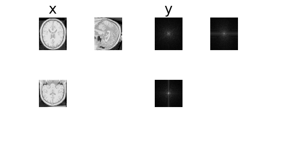
Here, we use a demo 3D brain volume of shape (181, 217, 181) from the
BrainWeb dataset
and simulate 3D single-coil or multi-coil Fourier measurements using
deepinv.physics.MRI or
deepinv.physics.MultiCoilMRI.
x = (
    torch.from_numpy(
        dinv.utils.demo.load_np_url(
            "https://huggingface.co/datasets/deepinv/images/resolve/main/brainweb_t1_ICBM_1mm_subject_0.npy?download=true"
        )
    )
    .unsqueeze(0)
    .unsqueeze(0)
    .to(device)
)
x = torch.cat([x, torch.zeros_like(x)], dim=1)  # add imaginary dimension

print(x.shape)  # (B, C, D, H, W) where D is depth

physics = dinv.physics.MultiCoilMRI(img_size=x.shape[1:], three_d=True, device=device)
physics = dinv.physics.MRI(img_size=x.shape[1:], three_d=True, device=device)

dinv.utils.plot_ortho3D([x, physics(x)], titles=["x", "y"])
torch.Size([1, 2, 181, 217, 181])
6. Explore dynamic MRI#
Finally, we show how to use the dynamic MRI for image sequence data of
shape (B, C, T, H, W) where T is the time dimension. Note that
this is also compatible with 3D MRI. We use dynamic MRI data from the
CMRxRecon challenge of cardiac cine
sequences and load them using deepinv.datasets.CMRxReconSliceDataset
provided in deepinv. We download demo data from the first patient
including ground truth images, undersampled kspace, and associated masks:
dinv.datasets.download_archive(
    dinv.utils.get_image_url("CMRxRecon.zip"),
    dinv.utils.get_data_home() / "CMRxRecon.zip",
    extract=True,
)

dataset = dinv.datasets.CMRxReconSliceDataset(
    dinv.utils.get_data_home() / "CMRxRecon",
)

x, y, params = next(iter(DataLoader(dataset)))

print(
    f"""
    Ground truth: {x.shape} (B, C, T, H, W)
    Measurements: {y.shape}
    Acc. mask: {params["mask"].shape}
"""
)
  0%|          | 0/24695321 [00:00<?, ?it/s]
100%|██████████| 23.6M/23.6M [00:00<00:00, 317MB/s]

Extracting:   0%|          | 0/10 [00:00<?, ?it/s]
Extracting: 100%|██████████| 10/10 [00:00<00:00, 128.92it/s]

  0%|          | 0/1 [00:00<?, ?it/s]
100%|██████████| 1/1 [00:00<00:00,  6.97it/s]
100%|██████████| 1/1 [00:00<00:00,  6.95it/s]

    Ground truth: torch.Size([1, 2, 12, 512, 256]) (B, C, T, H, W)
    Measurements: torch.Size([1, 2, 12, 512, 256])
    Acc. mask: torch.Size([1, 2, 1, 512, 256])
Dynamic MRI data is directly compatible with existing functionality.
For example, you can train with this data by passing the dataset to
deepinv.Trainer, which will automatically load in the data
x, y, params. Or, you can use the data directly with the physics
deepinv.physics.DynamicMRI.
You can also pass in a custom k-t acceleration mask generator to generate random time-varying masks:
physics_generator = dinv.physics.generator.EquispacedMaskGenerator(
    img_size=x.shape[1:], acceleration=16, rng=rng, device=device
)
physics = dinv.physics.DynamicMRI(img_size=(512, 256), device=device)

dataset = dinv.datasets.CMRxReconSliceDataset(
    dinv.utils.get_data_home() / "CMRxRecon",
    mask_generator=physics_generator,
    mask_dir=None,
)

x, y, params = next(iter(DataLoader(dataset)))
  0%|          | 0/1 [00:00<?, ?it/s]
100%|██████████| 1/1 [00:00<00:00,  7.08it/s]
100%|██████████| 1/1 [00:00<00:00,  7.07it/s]
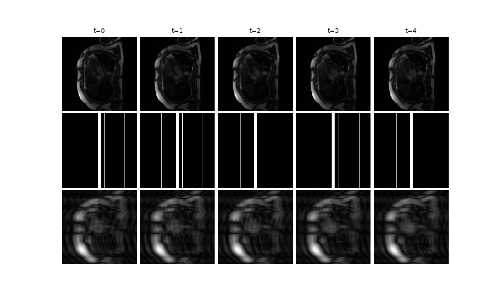
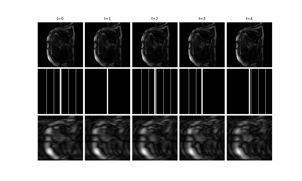
We provide a video plotting function, deepinv.utils.plot_videos. Here, we
visualise t=5 frames of the ground truth x, the mask, and the zero-filled
reconstruction x_zf (and crop to square for better visibility):
x_zf = physics.A_adjoint(y, **params)

dinv.utils.plot(
    {
        f"t={i}": torch.cat([x[:, :, i], params["mask"][:, :, i], x_zf[:, :, i]])[
            ..., 128:384, :
        ]
        for i in range(5)
    }
)
- References:
Total running time of the script: (0 minutes 5.044 seconds)


