plot#
- deepinv.utils.plot(img_list, titles=None, save_fn=None, save_dir=None, tight=True, max_imgs=4, rescale_mode='min_max', show=True, close=False, figsize=None, subtitles=None, suptitle=None, cmap='gray', fontsize=None, interpolation='none', cbar=False, dpi=1200, fig=None, axs=None, return_fig=False, return_axs=False, vmin=None, vmax=None, labels=None, label_loc=(0.03, 0.03), plot_inset=False, extract_loc=(0.0, 0.0), extract_size=0.2, inset_loc=(0.0, 0.5), inset_size=0.4, **imshow_kwargs)[source]#
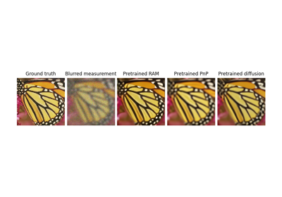
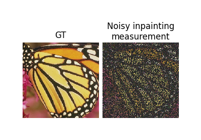
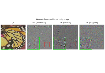
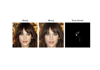
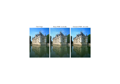
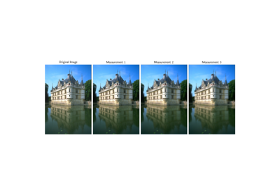
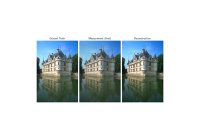
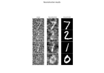
Plots a list of images.
The images should be of shape [B,C,H,W] or [C, H, W], where B is the batch size, C is the number of channels, H is the height and W is the width. The images are plotted in a grid, where the number of rows is B and the number of columns is the length of the list. If the B is bigger than max_imgs, only the first batches are plotted.
Warning
If the number of channels is 2, the magnitude of the complex images is plotted. If the number of channels is bigger than 3, only the first 3 channels are plotted.
We provide flexibility to save plots either side-by-side using
save_fnor as individual images usingsave_dir.Note
Zoomed-in insets can be plotted by setting
plot_inset=True. Seeplot_inset()for the original implementation.Example usage:
import torch
from deepinv.utils import plot
img = torch.rand(4, 3, 256, 256)
plot([img, img, img], titles=["img1", "img2", "img3"], save_dir="test.png")
Note
Using
show=Truecallsplt.show()with blocking (outside notebook environments). If this is undesired simply usefig = plot(..., show=False, return_fig=True)and plot at your desired location usingfig.show().- Parameters:
img_list (list[torch.Tensor], dict[str,torch.Tensor], torch.Tensor) – list of images, single image, or dict of titles: images to plot.
titles (list[str], str, None) – list of titles for each image, has to be same length as img_list.
save_fn (None, str, pathlib.Path) – path to save the plot as a single image (i.e. side-by-side).
save_dir (None, str, pathlib.Path) – path to save the plots as individual images.
tight (bool) – use tight layout.
max_imgs (int) – maximum number of images to plot.
rescale_mode (str) – rescale mode, either
'min_max'(images are linearly rescaled between 0 and 1 using their min and max values) or'clip'(images are clipped between 0 and 1).show (bool) – show the image plot. Under the hood, this calls the
plt.show()function.close (bool) – close the image plot. Under the hood, this calls the
plt.close()function.figsize (tuple[int]) – size of the figure. If
None, calculated from the size ofimg_list.subtitles (list[list[str]], list[str], str, None) – list of subtitles for each image, can be either the same length or the same shape as img_list.
suptitle (str) – title of the figure.
cmap (str) – colormap to use for the images. Default: gray
interpolation (str) – interpolation to use for the images. See https://matplotlib.org/stable/gallery/images_contours_and_fields/interpolation_methods.html for more details. Default: none
dpi (int) – DPI to save images.
fig (None, matplotlib.figure.Figure) – matplotlib Figure object to plot on. If None, create new Figure. Defaults to None.
axs (None, matplotlib.axes.Axes) – matplotlib Axes object to plot on. If None, create new Axes. Defaults to None.
return_fig (bool) – return the figure object.
return_axs (bool) – return the axs object.
vmin (float, None) – minimum value for clipping when using ‘clip’ rescaling.
vmax (float, None) – maximum value for clipping when using ‘clip’ rescaling.
labels (list[str], None) – list of overlaid labels for each image, has to be same length as img_list.
label_loc (tuple, list) – location or locations for label to be plotted on image. Defaults to (.03, .03). Coordinates are fractions from 0-1, where (0, 0) is the top left corner and (1, 1) is the bottom right corner.
plot_inset (bool) – whether to plot zoomed-in insets. Defaults to False.
extract_loc (tuple, list) – image location or locations for extract to be taken from. Defaults to (0., 0.). Coordinates are fractions from 0-1, where (0, 0) is the top left corner and (1, 1) is the bottom right corner.
extract_size (float) – size of extract to be taken from image. Defaults to 0.2.
inset_loc (tuple, list) – location or locations for inset to be plotted on image. Defaults to (0., 0.5). Coordinates are fractions from 0-1, where (0, 0) is the top left corner and (1, 1) is the bottom right corner.
inset_size (float) – size of inset to be plotted on image. Defaults to 0.4.
imshow_kwargs – keyword args to pass to the matplotlib
imshowcalls. See imshow docs for possible kwargs.
Examples using plot:#
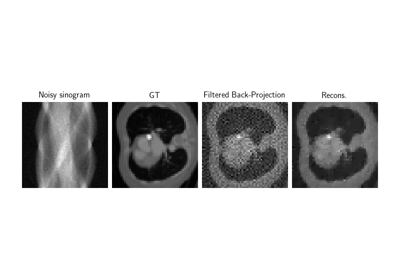
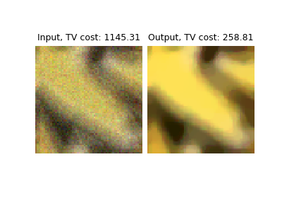
Low-dose CT with ASTRA backend and Total-Variation (TV) prior

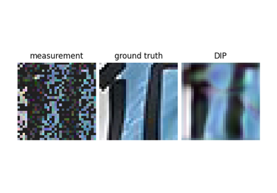
Reconstructing an image using the deep image prior.
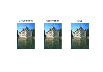
Expected Patch Log Likelihood (EPLL) for Denoising and Inpainting
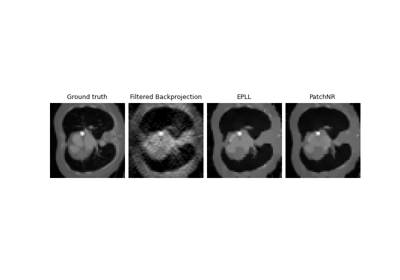
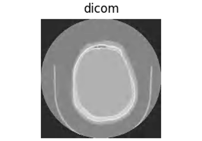
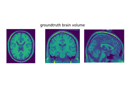
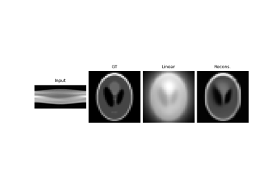
Patch priors for limited-angle computed tomography
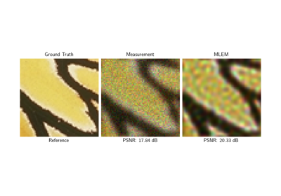
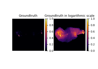
Poisson Inverse Problems with Maximum-Likelihood Expectation-Maximization (MLEM)

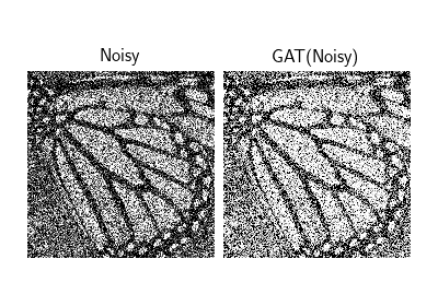
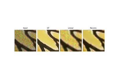
Poisson-Gaussian Denoising with the Generalized Anscombe Transform
Random phase retrieval and reconstruction methods.

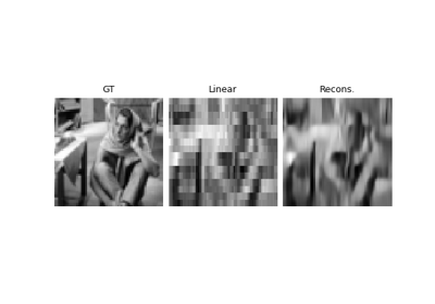
Pattern Ordering in a Compressive Single Pixel Camera
PnP with custom optimization algorithm (Primal-Dual Condat-Vu)
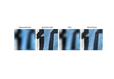
Plug-and-Play algorithm with Mirror Descent for Poisson noise inverse problems.
Using state-of-the-art diffusion models from HuggingFace Diffusers with DeepInverse
Building your diffusion posterior sampling method using SDEs

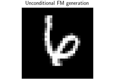
Flow-Matching for posterior sampling and unconditional generation

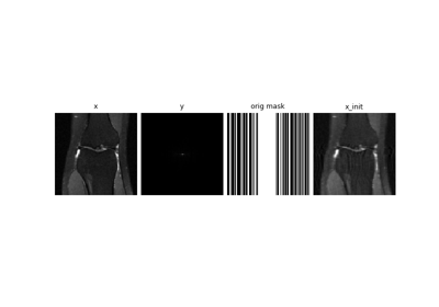
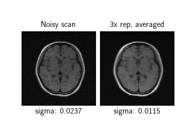
Self-supervised MRI reconstruction with Artifact2Artifact
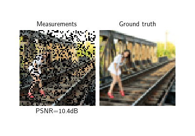
Self-supervised learning with Equivariant Splitting
Deep Equilibrium (DEQ) algorithms for image deblurring
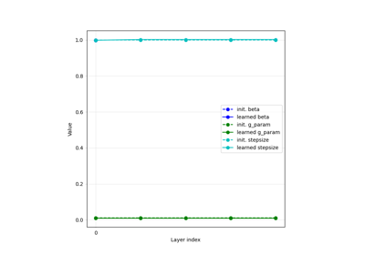
Learned Iterative Soft-Thresholding Algorithm (LISTA) for compressed sensing


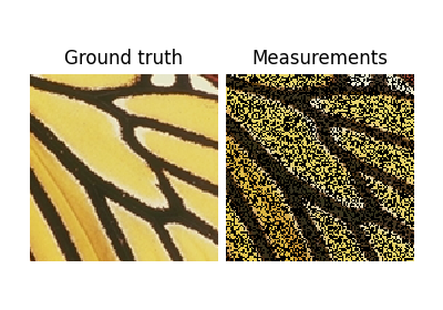
Unfolded Chambolle-Pock for constrained image inpainting