Training a reconstruction model

This example provides a very simple quick start introduction to training reconstruction networks with DeepInverse for solving imaging inverse problems.

Training requires these components, all of which you can define with DeepInverse:

• A model to be trained from reconstructors or define your own.

• A physics from our list of physics. Or, bring your own physics.

• A dataset of images and/or measurements from datasets. Or, bring your own dataset.

• A loss from our loss functions.

• A metric from our metrics.

Here, we demonstrate a simple experiment of training a UNet on an inpainting task on the Urban100 dataset of natural images.

import deepinv as dinv
import torch

device = dinv.utils.get_freer_gpu() if torch.cuda.is_available() else "cpu"
rng = torch.Generator(device=device).manual_seed(0)

Selected GPU 0 with 8215.25 MiB free memory

Setup

First, define the physics that we want to train on.

physics = dinv.physics.Inpainting((1, 64, 64), mask=0.8, device=device, rng=rng)

Then define the dataset. Here we simulate a dataset of measurements from Urban100.

Tip

See datasets for types of datasets DeepInverse supports: e.g. paired, ground-truth-free, single-image…

from torchvision.transforms import Compose, ToTensor, Resize, CenterCrop, Grayscale

dataset = dinv.datasets.Urban100HR(
    ".",
    download=True,
    transform=Compose([ToTensor(), Grayscale(), Resize(256), CenterCrop(64)]),
)

train_dataset, test_dataset = torch.utils.data.random_split(
    torch.utils.data.Subset(dataset, range(50)), (0.8, 0.2)
)

dataset_path = dinv.datasets.generate_dataset(
    train_dataset=train_dataset,
    test_dataset=test_dataset,
    physics=physics,
    device=device,
    save_dir=".",
    batch_size=1,
)

train_dataloader = torch.utils.data.DataLoader(
    dinv.datasets.HDF5Dataset(dataset_path, train=True), shuffle=True
)
test_dataloader = torch.utils.data.DataLoader(
    dinv.datasets.HDF5Dataset(dataset_path, train=False), shuffle=False
)

  0%|          | 0/135388067 [00:00<?, ?it/s]
  7%|▋         | 9.50M/129M [00:00<00:01, 99.1MB/s]
 16%|█▌        | 20.4M/129M [00:00<00:01, 103MB/s]
 25%|██▌       | 32.8M/129M [00:00<00:00, 115MB/s]
 34%|███▍      | 43.8M/129M [00:00<00:00, 112MB/s]
 43%|████▎     | 55.1M/129M [00:00<00:00, 114MB/s]
 52%|█████▏    | 66.7M/129M [00:00<00:00, 117MB/s]
 61%|██████    | 78.2M/129M [00:00<00:00, 118MB/s]
 69%|██████▉   | 89.4M/129M [00:00<00:00, 118MB/s]
 78%|███████▊  | 101M/129M [00:00<00:00, 117MB/s]
 87%|████████▋ | 112M/129M [00:01<00:00, 117MB/s]
 95%|█████████▌| 123M/129M [00:01<00:00, 117MB/s]
100%|██████████| 129M/129M [00:01<00:00, 115MB/s]

Extracting:   0%|          | 0/101 [00:00<?, ?it/s]
Extracting:   9%|▉         | 9/101 [00:00<00:01, 88.11it/s]
Extracting:  21%|██        | 21/101 [00:00<00:00, 99.90it/s]
Extracting:  33%|███▎      | 33/101 [00:00<00:00, 108.03it/s]
Extracting:  48%|████▊     | 48/101 [00:00<00:00, 123.84it/s]
Extracting:  60%|██████    | 61/101 [00:00<00:00, 117.51it/s]
Extracting:  72%|███████▏  | 73/101 [00:00<00:00, 108.32it/s]
Extracting:  83%|████████▎ | 84/101 [00:00<00:00, 107.06it/s]
Extracting:  94%|█████████▍| 95/101 [00:00<00:00, 107.71it/s]
Extracting: 100%|██████████| 101/101 [00:00<00:00, 109.44it/s]
Dataset has been successfully downloaded.
Dataset has been saved at ./dinv_dataset0.h5

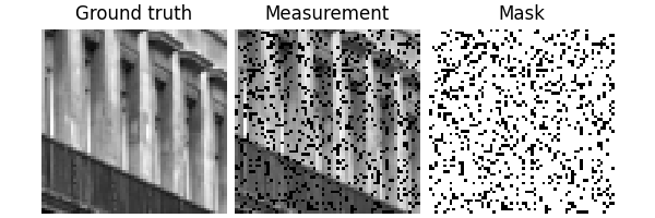
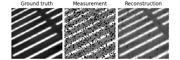
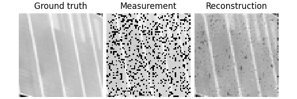
Visualize a data sample:

x, y = next(iter(test_dataloader))
dinv.utils.plot({"Ground truth": x, "Measurement": y, "Mask": physics.mask})

For the model we use an artifact removal model, where \(\phi_{\theta}\) is a U-Net

\[f_{\theta}(y) = \phi_{\theta}(A^{\top}(y))\]

model = dinv.models.ArtifactRemoval(
    dinv.models.UNet(1, 1, scales=2, batch_norm=False).to(device)
)

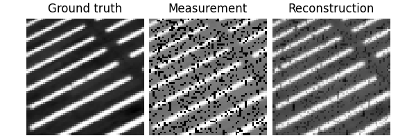
Train the model

We train the model using the deepinv.Trainer class, which cleanly handles all steps for training.

We perform supervised learning and use the mean squared error as loss function. See losses for all supported state-of-the-art loss functions.

We evaluate using the PSNR metric. See metrics for all supported metrics.

Note

In this example, we only train for a few epochs to keep the training time short. For a good reconstruction quality, we recommend to train for at least 100 epochs.

trainer = dinv.Trainer(
    model=model,
    physics=physics,
    optimizer=torch.optim.Adam(model.parameters(), lr=1e-3),
    train_dataloader=train_dataloader,
    eval_dataloader=test_dataloader,
    epochs=5,
    losses=dinv.loss.SupLoss(metric=dinv.metric.MSE()),
    metrics=dinv.metric.PSNR(),
    device=device,
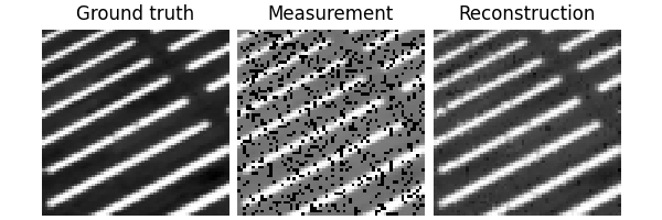
    plot_images=True,
    show_progress_bar=False,
)

_ = trainer.train()

• 
• 
• 
• 
• 
• 
• 
• 
• 
• 

/local/jtachell/deepinv/deepinv/deepinv/training/trainer.py:1352: UserWarning: non_blocking_transfers=True but DataLoader.pin_memory=False; set pin_memory=True to overlap host-device copies with compute.
  self.setup_train()
The model has 443585 trainable parameters
Train epoch 0: TotalLoss=0.016, PSNR=20.066
Eval epoch 0: PSNR=22.044
Best model saved at epoch 1
Train epoch 1: TotalLoss=0.004, PSNR=25.066
Eval epoch 1: PSNR=26.164
Best model saved at epoch 2
Train epoch 2: TotalLoss=0.002, PSNR=27.299
Eval epoch 2: PSNR=28.848
Best model saved at epoch 3
Train epoch 3: TotalLoss=0.001, PSNR=28.899
Eval epoch 3: PSNR=28.608
Train epoch 4: TotalLoss=0.001, PSNR=29.009
Eval epoch 4: PSNR=29.572
Best model saved at epoch 5

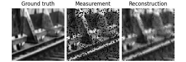
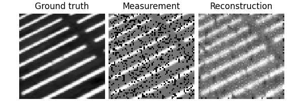
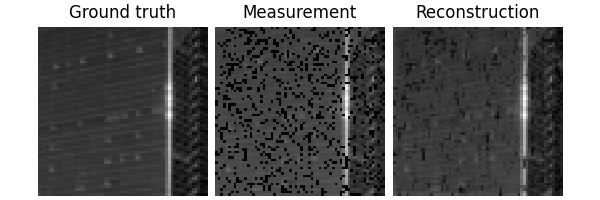
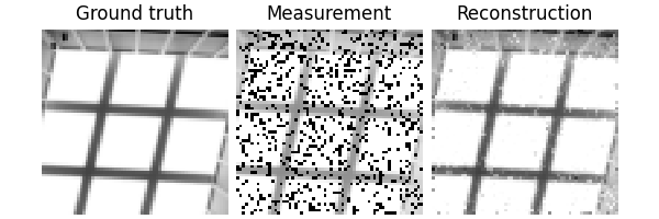
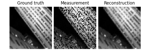
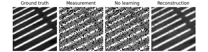
Test the network

We can now test the trained network using the deepinv.test() function.

The testing function will compute metrics and plot and save the results.

trainer.test(test_dataloader)

/local/jtachell/deepinv/deepinv/deepinv/training/trainer.py:1544: UserWarning: non_blocking_transfers=True but DataLoader.pin_memory=False; set pin_memory=True to overlap host-device copies with compute.
  self.setup_train(train=False)
Eval epoch 0: PSNR=29.572, PSNR no learning=12.979
Test results:
PSNR no learning: 12.979 +- 2.174
PSNR: 29.572 +- 2.114

{'PSNR no learning': 12.9794451713562, 'PSNR no learning_std': 2.1739899966255893, 'PSNR': 29.572228050231935, 'PSNR_std': 2.113502159331143}