Tour of forward sensing operators

This example provides a tour of some of the forward operators implemented in DeepInverse. We restrict ourselves to operators where the signal is a 2D image. The full list of operators can be found in here.

import torch

import deepinv as dinv
from deepinv.utils.plotting import plot
from deepinv.utils import load_example

Load image from the internet

This example uses an image of the CBSD68 dataset.

device = dinv.utils.get_freer_gpu() if torch.cuda.is_available() else "cpu"

x = load_example("CBSD_0010.png", grayscale=False).to(device)

x = torch.tensor(x, device=device, dtype=torch.float)
x = torch.nn.functional.interpolate(x, size=(64, 64))
img_size = x.shape[1:]
# Set the global random seed from pytorch to ensure reproducibility of the example.
torch.manual_seed(0)

/home/runner/work/deepinv/deepinv/examples/physics/demo_physics_tour.py:28: UserWarning: To copy construct from a tensor, it is recommended to use sourceTensor.clone().detach() or sourceTensor.clone().detach().requires_grad_(True), rather than torch.tensor(sourceTensor).
  x = torch.tensor(x, device=device, dtype=torch.float)

<torch._C.Generator object at 0x7f8135136290>

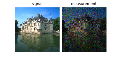
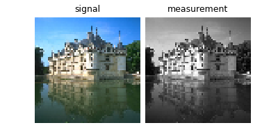
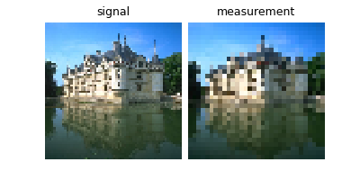
Denoising

The denoising class deepinv.physics.Denoising is associated with an identity operator. In this example we choose a Poisson noise.

physics = dinv.physics.Denoising(dinv.physics.PoissonNoise(0.1))

y = physics(x)

# plot results
plot([x, y], titles=["signal", "measurement"])

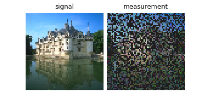
Inpainting

The inpainting class deepinv.physics.Inpainting is associated with a mask operator. The mask is generated at random (unless an explicit mask is provided as input). We also consider Gaussian noise in this example.

sigma = 0.1  # noise level
physics = dinv.physics.Inpainting(
    mask=0.5,
    img_size=x.shape[1:],
    noise_model=dinv.physics.GaussianNoise(sigma=sigma),
    device=device,
)

y = physics(x)

# plot results
plot([x, y], titles=["signal", "measurement"])

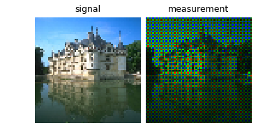
Demosaicing

The demosaicing class deepinv.physics.Demosaicing is associated with a Bayer pattern, which is a color filter array used in digital cameras (see Wikipedia).

physics = dinv.physics.Demosaicing(img_size=(64, 64), device=device)

y = physics(x)

# plot results
plot([x, y], titles=["signal", "measurement"])

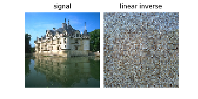
Compressed Sensing

The compressed sensing class deepinv.physics.CompressedSensing is associated with a random Gaussian matrix. Here we take 2048 measurements of an image of size 64x64, which corresponds to a compression ratio of 2.

physics = dinv.physics.CompressedSensing(
    m=2048,
    fast=False,
    channelwise=True,
    img_size=img_size,
    device=device,
)

y = physics(x)

# plot results
plot([x, physics.A_dagger(y)], titles=["signal", "linear inverse"])

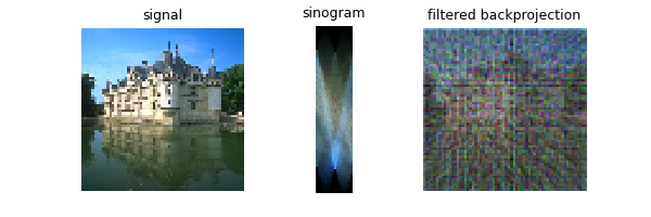
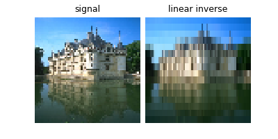
Computed Tomography

The class deepinv.physics.Tomography is associated with the sparse Radon transform. Here we take 20 views of an image of size 64x64, and consider mixed Poisson-Gaussian noise.

physics = dinv.physics.Tomography(
    img_width=img_size[-1],
    angles=20,
    device=device,
    noise_model=dinv.physics.PoissonGaussianNoise(gain=0.1, sigma=0.05),
)

y = physics(x)

# plot results
plot(
    [x, (y - y.min()) / y.max(), physics.A_dagger(y)],
    titles=["signal", "sinogram", "filtered backprojection"],
)

/home/runner/work/deepinv/deepinv/deepinv/physics/tomography.py:188: UserWarning: The default value of `normalize` is not specified and will be automatically set to `True`. Set `normalize` explicitly to `True` or `False` to avoid this warning.
  warn(
Power iteration converged at iteration 11, ||A^T A||_2=1236.31

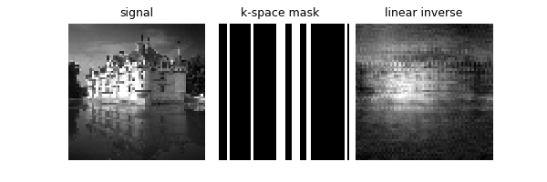
MRI

The class deepinv.physics.MRI is associated with a subsampling of the Fourier transform. The mask indicates which Fourier coefficients are measured. Here we use a random Cartesian mask, which corresponds to a compression ratio of approximately 4.

Note

The signal must be complex-valued for this operator, where the first channel corresponds to the real part and the second channel to the imaginary part. In this example, we set the imaginary part to zero.

mask = torch.rand((1, img_size[-1]), device=device) > 0.75
mask = torch.ones((img_size[-2], 1), device=device) * mask
mask[:, int(img_size[-1] / 2) - 2 : int(img_size[-1] / 2) + 2] = 1

physics = dinv.physics.MRI(
    mask=mask, device=device, noise_model=dinv.physics.GaussianNoise(sigma=0.05)
)

x2 = torch.cat(
    [x[:, 0, :, :].unsqueeze(1), torch.zeros_like(x[:, 0, :, :].unsqueeze(1))], dim=1
)
y = physics(x2)

# plot results
plot(
    [x2, mask.unsqueeze(0).unsqueeze(0), physics.A_adjoint(y)],
    titles=["signal", "k-space mask", "linear inverse"],
)

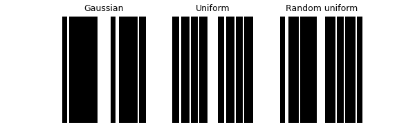
We also provide physics generators for various accelerated MRI masks. These are Cartesian sampling strategies and can be used for static (k) and dynamic (k-t) undersampling:

from deepinv.physics.generator import (
    GaussianMaskGenerator,
    RandomMaskGenerator,
    EquispacedMaskGenerator,
)

# shape (C, T, H, W)
mask_gaussian = GaussianMaskGenerator((2, 8, 64, 50), acceleration=4).step()["mask"]
mask_uniform = EquispacedMaskGenerator((2, 8, 64, 50), acceleration=4).step()["mask"]
mask_random = RandomMaskGenerator((2, 8, 64, 50), acceleration=4).step()["mask"]

plot(
    [
        mask_gaussian[:, :, 0, ...],
        mask_uniform[:, :, 0, ...],
        mask_random[:, :, 0, ...],
    ],
    titles=["Gaussian", "Uniform", "Random uniform"],
)

Decolorize

The class deepinv.physics.Decolorize is associated with a simple color-to-gray operator.

physics = dinv.physics.Decolorize(device=device)

y = physics(x)

# plot results
plot([x, y], titles=["signal", "measurement"])

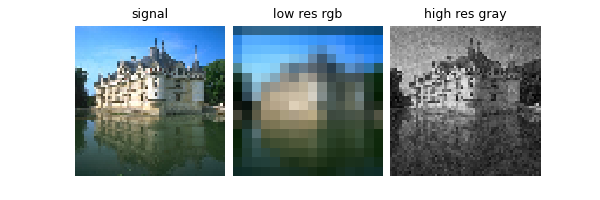
Pan-sharpening

The class deepinv.physics.Pansharpen obtains measurements which consist of a high-resolution grayscale image and a low-resolution RGB image.

physics = dinv.physics.Pansharpen(img_size=img_size, device=device)

y = physics(x)

# plot results
plot([x, y[0], y[1]], titles=["signal", "low res rgb", "high res gray"])

Single-Pixel Camera

The single-pixel camera class deepinv.physics.SinglePixelCamera is associated with m binary patterns. When fast=True, the patterns are generated using a fast Hadamard transform.

physics = dinv.physics.SinglePixelCamera(
    m=1024, fast=True, ordering="cake_cutting", img_size=img_size, device=device
)

y = physics(x)

# plot results
plot([x, physics.A_adjoint(y)], titles=["signal", "linear inverse"])

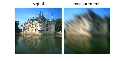
Blur

The class deepinv.physics.Blur blurs the input image with a specified kernel. Here we use a Gaussian blur with a standard deviation of 2 pixels and an angle of 45 degrees.

physics = dinv.physics.Blur(
    dinv.physics.blur.gaussian_blur(sigma=(2, 0.1), angle=45.0), device=device
)

y = physics(x)

# plot results
plot([x, y], titles=["signal", "measurement"])

Super-Resolution

The downsampling class deepinv.physics.Downsampling is associated with a downsampling operator.

physics = dinv.physics.Downsampling(
    img_size=img_size, factor=2, device=device, filter="bicubic"
)


y = physics(x)

# plot results
plot([x, y], titles=["signal", "measurement"])