Pattern Ordering in a Compressive Single Pixel Camera

This demo illustrates the impact of different Hadamard pattern ordering algorithms in the Single Pixel Camera (SPC), a computational imaging system that uses a single photodetector to capture images by projecting the scene onto a series of patterns. The SPC is implemented in the DeepInverse library.

In this example, we explore the following ordering algorithms for the Hadamard transform:

1. Sequency Ordering: Rows are ordered based on the number of sign changes (sequency pattern). Reference: https://en.wikipedia.org/wiki/Walsh_matrix#Sequency_ordering

2. Cake Cutting Ordering: Rows are ordered based on the number of blocks in the 2D resized Hadamard matrix [1].

3. Zig-Zag Ordering: Rows are ordered in a zig-zag pattern from the top-left to the bottom-right of the matrix [2].

4. XY Ordering: Rows are ordered in a circular pattern starting from the top-left to the bottom-right [3].

We compare the reconstructions obtained using these orderings and visualize their corresponding masks and Hadamard spectrum.

import torch
from pathlib import Path
import deepinv as dinv
from deepinv.utils import get_image_url, load_url_image
from deepinv.utils.plotting import plot
from deepinv.loss.metric import PSNR
from deepinv.physics.singlepixel import hadamard_2d_shift

General Setup

BASE_DIR = Path(".")
RESULTS_DIR = BASE_DIR / "results"

# Set the global random seed for reproducibility.
torch.manual_seed(0)
device = dinv.utils.get_device()

Selected CPU device

Configuration

Define the image size, noise level, number of measurements, and ordering algorithms.

img_size_H = 128  # Size of the image (128x128 pixels)
img_size_W = 128
noise_level_img = 0.0  # Noise level in the image
n = img_size_H * img_size_W  # Total number of pixels in the image
m = 5000  # Number of measurements
orderings = [
    "sequency",
    "cake_cutting",
    "zig_zag",
    "xy",
]  # Ordering algorithms to compare

Load Image

Load a grayscale image from the internet and resize it to the desired size.

url = get_image_url("barbara.jpeg")
x = load_url_image(
    url=url,
    img_size=(img_size_H, img_size_W),
    grayscale=True,
    resize_mode="resize",
    device=device,
)

Create Physics Models

Instantiate Single Pixel Camera models with different ordering algorithms.

physics_list = [
    dinv.physics.SinglePixelCamera(
        m=m,
        img_size=(1, img_size_H, img_size_W),
        noise_model=dinv.physics.GaussianNoise(sigma=noise_level_img),
        device=device,
        ordering=ordering,
    )
    for ordering in orderings
]

Generate Measurements and Reconstructions

Generate measurements using the physics models and reconstruct images using the adjoint operator.

y_list = [physics(x) for physics in physics_list]
x_list = [physics.A_adjoint(y) for physics, y in zip(physics_list, y_list, strict=True)]

Calculate PSNR

Compute the Peak Signal-to-Noise Ratio (PSNR) for each reconstruction.

psnr_metric = PSNR()
psnr_values = [psnr_metric(x_recon, x).item() for x_recon in x_list]

# Prepare titles for plotting
title_orderings = [o.replace("_", " ").title() for o in orderings]
title_orderings[-1] = "XY"  # Special case for 'xy'
titles = ["Ground Truth"] + title_orderings
subtitles = ["PSNR"] + [f"{psnr:.2f} dB" for psnr in psnr_values]
# Print information about the SPC setup
undersampling_rate = physics_list[0].mask.sum().float() / n
print(f"Image Size: {x.shape}")
print(f"SPC Measurements: {physics_list[0].mask.sum()}")
print(f"SPC Undersampling Rate: {undersampling_rate:.2f}")

Image Size: torch.Size([1, 1, 128, 128])
SPC Measurements: 5000.0
SPC Undersampling Rate: 0.31

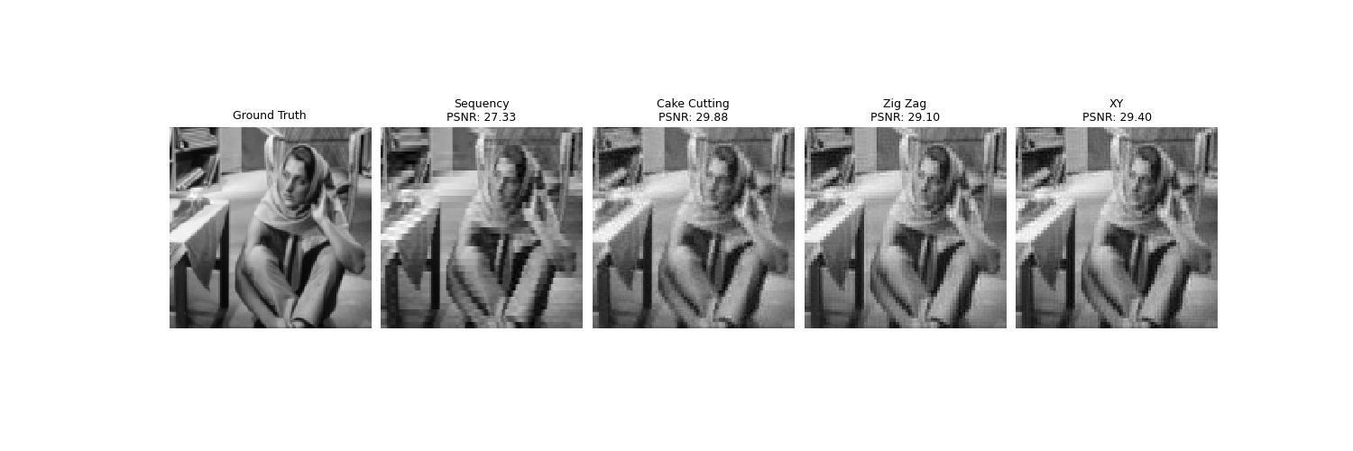
Plot Reconstructions

Visualize the ground truth and reconstructed images with PSNR values.

plot(
    [x] + x_list,
    titles=titles,
    subtitles=subtitles,
    show=True,
    figsize=(15, 5),
    fontsize=24,
)

# Recovery Algorithm
# ------------------
# Use a Plug-and-Play (PnP) denoising prior with the ADMM optimization algorithm for image recovery.
from deepinv.models import DnCNN
from deepinv.optim.data_fidelity import L2
from deepinv.optim.prior import PnP
from deepinv.optim import ADMM

n_channels = 1  # Number of channels in the image

# Define the data fidelity term (L2 loss)
data_fidelity = L2()

# Specify the denoising prior using a pretrained DnCNN model
denoiser = DnCNN(
    in_channels=n_channels,
    out_channels=n_channels,
    pretrained="download",  # Automatically downloads pretrained weights
    device=device,
)

# Define the prior using the Plug-and-Play framework
prior = PnP(denoiser=denoiser)

# Set optimization parameters
max_iter = 5  # Maximum number of iterations
noise_level_img = 0.03  # Noise level in the image
stepsize = 0.8  # Step size for the optimization

model = ADMM(
    prior=prior,
    data_fidelity=data_fidelity,
    early_stop=False,
    max_iter=max_iter,
    verbose=False,
    stepsize=stepsize,
    sigma_denoiser=noise_level_img,
    g_first=True,
)

# Set the model to evaluation mode (no training required)
model.eval()

# Perform image reconstruction using the optimization algorithm
x_recon = []
psnr_values = []

for y, physics in zip(y_list, physics_list, strict=True):
    x_recon.append(model(y, physics))
    psnr_values.append(psnr_metric(x_recon[-1], x).item())

# Update titles with PSNR values for the reconstructed images
titles = ["Ground Truth"] + title_orderings
subtitles = ["PSNR"] + [f"{psnr:.2f} dB" for psnr in psnr_values]

Plot ADMM-TV Reconstructions

Visualize the ground truth and reconstructed images with PSNR values.

plot(
    [x] + x_recon,
    titles=titles,
    subtitles=subtitles,
    show=True,
    figsize=(15, 5),
    fontsize=24,
)

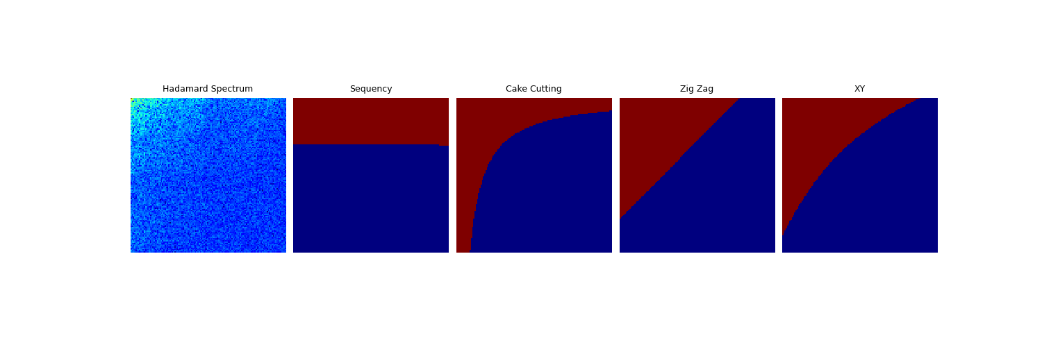
Visualize Masks and Hadamard Spectrum

Prepare and plot masks and the Hadamard spectrum for visualization.

masks = [physics.mask for physics in physics_list]
shifted_masks = [hadamard_2d_shift(mask) for mask in masks]

# Calculate the Hadamard spectrum for visualization
physics_full = dinv.physics.SinglePixelCamera(
    m=n,
    img_size=(1, img_size_H, img_size_W),
    noise_model=dinv.physics.GaussianNoise(sigma=noise_level_img),
    device=device,
)
y_spectrum = hadamard_2d_shift(physics_full(x))
y_spectrum = torch.pow(torch.abs(y_spectrum), 0.2)
y_spectrum = y_spectrum / y_spectrum.max()

# Plot the masks and Hadamard spectrum
plot(
    [y_spectrum] + shifted_masks,
    titles=["Hadamard Spectrum"] + title_orderings,
    show=True,
    figsize=(15, 5),
    cmap="jet",
    fontsize=24,
)

References:

[1]

Wen-Kai Yu. Super sub-nyquist single-pixel imaging by means of cake-cutting hadamard basis sort. Sensors, 19(19):4122, 2019.

[2]

Lourdes López-García, William Cruz-Santos, Anmi García-Arellano, Pedro Filio-Aguilar, José A Cisneros-Martínez, and Rubén Ramos-García. Efficient ordering of the hadamard basis for single pixel imaging. Optics Express, 30(8):13714–13732, 2022.

[3]

Yan Cai, Shijian Li, Wei Zhang, Hao Wu, Xuri Yao, and Qing Zhao. A detail-enhanced sampling strategy in hadamard single-pixel imaging. Chinese Optics Letters, 21(7):071101, 2023.