Reducing the memory and computational complexity of unfolded network training

Some unfolded architectures rely on a least-squares solver to compute the proximal step w.r.t. the data-fidelity term (e.g., ADMM or HQS):

\[\operatorname{prox}_{\gamma f}(z) = \underset{x}{\arg\min} \; \frac{\gamma}{2}\|A_\theta x-y\|^2 + \frac{1}{2}\|x-z\|^2\]

During backpropagation, a naive implementation requires storing the gradients of every intermediate step of the least squares solver (which is an iterative method), resulting in significant memory and computational costs which are proportional to number of iterations done by the solver.

The library provides a memory-efficient back-propagation strategy that reduces the memory footprint during training, by computing the gradients of the proximal step in closed-form, without storing any intermediate steps. This closed-form computation requires evaluating the least-squares solver one additional time during the gradient computation.

Let \(h(z, y, \theta, \gamma) = \operatorname{prox}_{\gamma f}(z)\) be the proximal operator. During the backward pass, we need to compute the vector-Jacobian products (VJPs), w.r.t the input variables \((z, y, \theta, \gamma)\) required for backpropagation:

\[\left( \frac{\partial h}{\partial z} \right)^{\top} v, \quad \left( \frac{\partial h}{\partial y} \right)^{\top} v, \quad \left( \frac{\partial h}{\partial \theta} \right)^{\top} v, \quad \left( \frac{\partial h}{\partial \gamma} \right)^{\top} v\]

and \(v\) is the upstream gradient. The VJPs can be computed in closed-form by solving a second least-squares problem, as shown in the following. When the forward least-squares solver converges to the exact minimizer, we have the following closed-form expressions for \(h(z, y, \theta, \gamma)\):

\[h(z, y, \theta, \gamma) = \left( A_\theta^{\top} A_\theta + \frac{1}{\gamma} I \right)^{-1} \left( A_\theta^{\top} y + \frac{1}{\gamma} z \right)\]

Let \(M\) denote the inverse \(\left( A_\theta^T A_\theta + \frac{1}{\gamma} I \right)^{-1}\). The VJPs can be computed as follows:

\[\begin{split}\left( \frac{\partial h}{\partial z} \right)^{\top} v &= \frac{1}{\gamma} M v \\ \left( \frac{\partial h}{\partial y} \right)^{\top} v &= A_\theta M v \\ \left( \frac{\partial h}{\partial \gamma} \right)^{\top} v &= (h - z)^\top M v / \gamma^2 \\ \left( \frac{\partial h}{\partial \theta} \right)^{\top} v &= \frac{\partial p}{\partial \theta}\end{split}\]

where \(p = (y - A_\theta h)^{\top} A_\theta M v ` and :math:\)frac{partial p}{partial theta}` can be computed using the standard backpropagation mechanism (autograd).

Note

Linear forward operators that have a closed-form singular value decomposition benefit from a closed-form formula for computing the proximal step, and thus we shouldn’t expect speed-ups in these specific cases.

This example shows how to train an unfolded neural network with a memory complexity that is independent of the number of iterations in least squares solver (O(1) memory complexity) used for computing the data-fidelity proximal step.

Note

By default, this example is run on CPU so we should not expect significant speed-ups and we can not trace the memory usage precisely. For a better experience, we recommend running the example on a machine with a GPU. In such a case, we can expect significant speed-ups (20-50%) and a significant reduction in memory usage (2x-3x reduction factor).

import deepinv as dinv
import torch
from torch.utils.data import DataLoader
from deepinv.optim.data_fidelity import L2
from deepinv.optim.prior import PnP
from deepinv.unfolded import unfolded_builder
from torchvision import transforms
from deepinv.utils.demo import load_dataset
import time
import numpy as np
import matplotlib.pyplot as plt

device = (
    dinv.utils.get_freer_gpu() if torch.cuda.is_available() else torch.device("cpu")
)
dtype = torch.float32
img_size = 64 if torch.cuda.is_available() else 32
num_images = 480 if torch.cuda.is_available() else 64

Define the degradation operator and the dataset.

We use the Blur class with valid padding from the physics module. ITs proximal operator does not have a closed-form solution, and thus requires using a least-squares solver.

# In this example, we use the CBSD500 dataset
train_dataset_name = "CBSD500"

# Specify the transforms to be applied to the input images.
train_transform = transforms.Compose(
    [transforms.RandomCrop(img_size), transforms.ToTensor()]
)
# Define the base train dataset of clean images.
train_dataset = load_dataset(train_dataset_name, transform=train_transform)
train_dataset = torch.utils.data.Subset(train_dataset, range(num_images))
train_loader = DataLoader(
    train_dataset,
    batch_size=32 if torch.cuda.is_available() else 8,
    num_workers=4 if torch.cuda.is_available() else 0,
    shuffle=True,
)
physics = dinv.physics.Blur(
    filter=dinv.physics.blur.gaussian_blur(sigma=(2.5, 2.5)),
    padding="valid",
    device=device,
    noise_model=dinv.physics.GaussianNoise(sigma=0.1),
    max_iter=100,
    tol=1e-8,
    implicit_backward_solver=False,
)

Define the unfolded parameters.

# Unrolled optimization algorithm parameters
max_iter = 5  # number of unfolded layers

# Select the data fidelity term
data_fidelity = L2()
stepsize = [1] * max_iter  # stepsize of the algorithm
sigma_denoiser = [0.01] * max_iter  # noise level parameter of the denoiser
params_algo = {  # wrap all the restoration parameters in a 'params_algo' dictionary
    "stepsize": stepsize,
    "g_param": sigma_denoiser,
}
trainable_params = [
    "g_param",
    "stepsize",
]  # define which parameters from 'params_algo' are trainable

Train the network

Here we write explicitly the training loop to show how implicit differentiation can be used to avoid out-of-memory issues and sometimes accelerate training. But you can also use the deepinv.Trainer class as shown in other examples.

# Some helper functions for measuring memory usage
use_cuda = device.type == "cuda" and torch.cuda.is_available()


def sync():
    if use_cuda:
        torch.cuda.synchronize()


def reset_memory():
    if use_cuda:
        torch.cuda.empty_cache()
        torch.cuda.reset_peak_memory_stats()


def peak_memory():
    if use_cuda:
        peak_bytes = int(torch.cuda.max_memory_allocated(device=device))
    else:  # Stats on CPU is not very accurate
        peak_bytes = 0
    return peak_bytes

We first train the model will full backpropagation to compare the memory usage. Define the unfolded trainable model.

torch.manual_seed(42)  # Make sure that we have the same initialization for both runs
prior = PnP(denoiser=dinv.models.DnCNN(depth=7, pretrained=None).to(device))
model = unfolded_builder(
    iteration="HQS",
    params_algo=params_algo.copy(),
    trainable_params=trainable_params,
    data_fidelity=data_fidelity,
    max_iter=max_iter,
    prior=prior,
).to(device)

optimizer = torch.optim.Adam(model.parameters(), lr=5e-4, weight_decay=1e-8)
model.train()

# Setting this parameter to False to use full backpropagation
physics.implicit_backward_solver = False

reset_memory()
sync()
start = time.perf_counter()
auto_losses = []
for x in train_loader:
    x = x.to(device)
    y = physics(x)
    optimizer.zero_grad()
    x_hat = model(physics=physics, y=y)
    loss = torch.nn.functional.mse_loss(x_hat, x)
    auto_losses.append(loss.item())
    loss.backward()
    optimizer.step()
sync()
end = time.perf_counter()
auto_peak_memory_mb = peak_memory() / (10**6)
auto_time_per_iter = (end - start) / len(train_loader)
auto_avg_loss = np.array(auto_losses)
auto_avg_loss = np.cumsum(auto_avg_loss) / (np.arange(len(auto_avg_loss)) + 1)

We now train the model using the closed-form gradients of the proximal step. We can do this by setting implicit_backward_solver to True.

physics.implicit_backward_solver = True

# Define the unfolded trainable model.
torch.manual_seed(42)  # Make sure that we have the same initialization for both runs
prior = PnP(denoiser=dinv.models.DnCNN(depth=7, pretrained=None).to(device))
model = unfolded_builder(
    iteration="HQS",
    params_algo=params_algo.copy(),
    trainable_params=trainable_params,
    data_fidelity=data_fidelity,
    max_iter=max_iter,
    prior=prior,
).to(device)

optimizer = torch.optim.Adam(model.parameters(), lr=5e-4, weight_decay=1e-8)
model.train()

reset_memory()
sync()
start = time.perf_counter()
implicit_losses = []
for x in train_loader:
    x = x.to(device)
    y = physics(x)
    optimizer.zero_grad()
    x_hat = model(physics=physics, y=y)
    loss = torch.nn.functional.mse_loss(x_hat, x)
    implicit_losses.append(loss.item())
    loss.backward()
    optimizer.step()
sync()
end = time.perf_counter()
implicit_peak_memory_mb = peak_memory() / (10**6)
implicit_time_per_iter = (end - start) / len(train_loader)
implicit_avg_loss = np.array(implicit_losses)
implicit_avg_loss = np.cumsum(implicit_avg_loss) / (
    np.arange(len(implicit_avg_loss)) + 1
)

Compare the memory usage

print(f"Full backpropagation: time per iteration: {auto_time_per_iter:.2f} s. ")
print(f"Implicit differentiation: time per iteration: {implicit_time_per_iter:.2f} s.")

# Compare the memory usage
if use_cuda:
    print(f"Full backpropagation: peak memory usage: {auto_peak_memory_mb:.1f} MB")
    print(
        f"Implicit differentiation: peak memory usage: {implicit_peak_memory_mb:.1f} MB"
    )
    print(
        f"Memory reduction factor: {auto_peak_memory_mb/implicit_peak_memory_mb:.1f}x"
    )


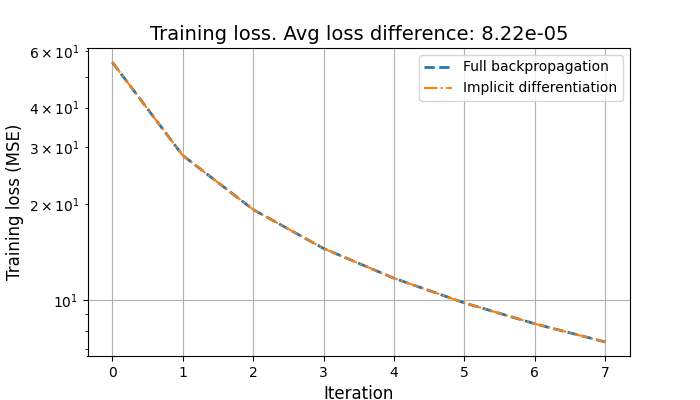
# Compare the training loss
plt.figure(figsize=(7, 4))
plt.plot(auto_avg_loss, label="Full backpropagation", linestyle="--", linewidth=2)
plt.plot(
    implicit_avg_loss, label="Implicit differentiation", linestyle="-.", linewidth=1.5
)
plt.yscale("log")
plt.xlabel("Iteration", fontsize=12)
plt.ylabel("Training loss (MSE)", fontsize=12)
plt.legend()
plt.title(
    f"Training loss. Avg loss difference: {np.mean(np.abs(auto_avg_loss - implicit_avg_loss)):.2e}",
    fontsize=14,
)
plt.grid()
plt.show()

Full backpropagation: time per iteration: 0.97 s.
Implicit differentiation: time per iteration: 0.89 s.