Ptychography phase retrieval

This example shows how to create a Ptychography phase retrieval operator and generate phaseless measurements from a given image.

General setup

Imports the necessary libraries and modules, including ptychography phase retrieval function from deepinv. It sets the device to GPU if available, otherwise uses the CPU.

import matplotlib.pyplot as plt
import torch
import numpy as np
import deepinv as dinv
from deepinv.utils.demo import load_example
from deepinv.utils.plotting import plot
from deepinv.physics import Ptychography
from deepinv.optim.data_fidelity import L1
from deepinv.optim.phase_retrieval import correct_global_phase

device = dinv.utils.get_freer_gpu() if torch.cuda.is_available() else "cpu"

Load image from the internet

Loads a sample image from a URL, resizes it to 128x128 pixels, and extracts only one color channel.

size = 128
image = load_example("CBSD_0010.png", grayscale=False, img_size=(size, size))

x = image[:, 0, ...].unsqueeze(1)  # Take only one channel
print(x.shape)
plot([x], figsize=(10, 10))

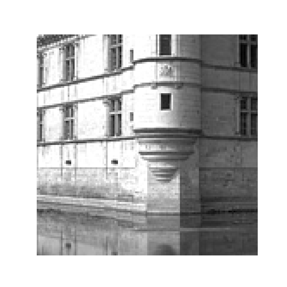
torch.Size([1, 1, 128, 128])

Prepare phase input

We use the original image as the phase information for the complex signal. The original value range is [0, 1], and we map it to the phase range [0, pi].

phase = x / x.max() * np.pi  # between 0 and pi
input = torch.exp(1j * phase.to(torch.complex64)).to(device)

Set up ptychography physics model

Initializes the ptychography physics model with parameters like the probe and shifts. This model will be used to simulate ptychography measurements.

img_size = (1, size, size)
n_img = 10**2
probe = dinv.physics.phase_retrieval.build_probe(
    img_size, type="disk", probe_radius=30, device=device
)
shifts = dinv.physics.phase_retrieval.generate_shifts(img_size, n_img=n_img, fov=170)

physics = Ptychography(
    img_size=img_size,
    probe=probe,
    shifts=shifts,
    device=device,
)

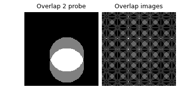
Display probe overlap

Calculates and displays the overlap of probe regions in the image, helping visualize the ptychography pattern.

overlap_img = physics.B.get_overlap_img(physics.B.shifts).cpu()
overlap2probe = physics.B.get_overlap_img(physics.B.shifts[55:57]).cpu()
plot(
    [overlap2probe.unsqueeze(0), overlap_img.unsqueeze(0)],
    titles=["Overlap 2 probe", "Overlap images"],
)

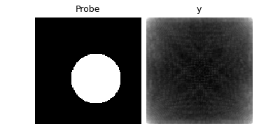
Generate and visualize probe and measurements

Displays the ptychography probe and a sum of the generated measurement data.

probe = physics.probe[:, 55].cpu()
y = physics(input)
plot(
    [torch.abs(probe), y[0].sum(dim=0).log().unsqueeze(0)],
    titles=["Probe", "y"],
)

Gradient descent for phase retrieval

Implements a simple gradient descent algorithm to minimize the L1 data fidelity loss for phase retrieval.

data_fidelity = L1()
lr = 0.1
n_iter = 200
x_est = torch.randn_like(x).to(device)
loss_hist = []

for i in range(n_iter):
    x_est = x_est - lr * data_fidelity.grad(x_est, y, physics)
    loss_hist.append(data_fidelity(x_est, y, physics).cpu())
    if i % 10 == 0:
        print(f"Iter {i}, loss: {loss_hist[i]}")

# Plot the loss curve
plt.plot(loss_hist)
plt.title("loss curve (gradient descent with random initialization)")
plt.show()

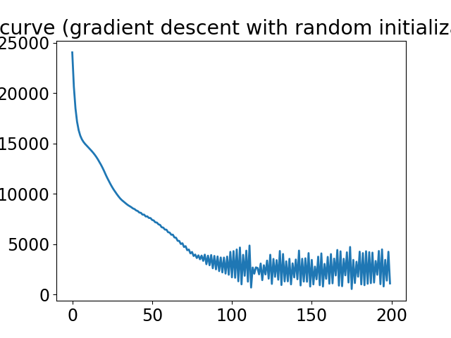
Iter 0, loss: tensor([23827.2051])
Iter 10, loss: tensor([14753.7051])
Iter 20, loss: tensor([12876.2285])
Iter 30, loss: tensor([7306.3105])
Iter 40, loss: tensor([4774.6973])
Iter 50, loss: tensor([4334.4370])
Iter 60, loss: tensor([3739.9526])
Iter 70, loss: tensor([3364.8022])
Iter 80, loss: tensor([4279.6562])
Iter 90, loss: tensor([3455.1978])
Iter 100, loss: tensor([4690.6206])
Iter 110, loss: tensor([2329.2983])
Iter 120, loss: tensor([4236.4712])
Iter 130, loss: tensor([4202.0352])
Iter 140, loss: tensor([3585.7258])
Iter 150, loss: tensor([3818.7305])
Iter 160, loss: tensor([2961.7820])
Iter 170, loss: tensor([3946.4189])
Iter 180, loss: tensor([4420.5371])
Iter 190, loss: tensor([3518.5283])

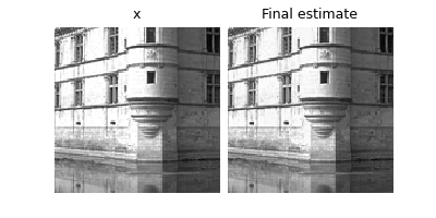
Display final estimated phase retrieval

Corrects the global phase of the estimated image to match the original phase and plots the result. This final visualization shows the original image and the estimated phase after retrieval.

x_est = x_est.detach().cpu()
final_est = correct_global_phase(x_est, x)
plot([x, torch.angle(final_est)], titles=["x", "Final estimate"])