Bring your own physics

This examples shows you how to use DeepInverse with your own physics.

While DeepInverse offers a large number of forward operators, you can also bring your own forward operator for your specific imaging problem.

DeepInverse’s modular physics framework makes this easy by letting you inherit useful methods from the most appropriate physics base class:

• deepinv.physics.Physics for non-linear operators;

• deepinv.physics.LinearPhysics for linear operators;

• deepinv.physics.DecomposablePhysics for linear operators with a closed-form singular value decomposition.

See also

Often your physics can be modelled without much work. You could:

• Use an existing physics but with custom params, e.g. blur with a custom kernel, or MRI with a custom sampling pattern. See parameter dependent operators.

• Inherit from an existing physics but override or wrap a particular method e.g. deepinv.physics.MRI \(\rightarrow\) deepinv.physics.DynamicMRI

• Define a new operator by combining existing operators.

In this example we will demonstrate creating a simple forward operator from scratch that converts RGB images to grayscale images. We also show you how to exploit the singular value decomposition of the operator to speed up the evaluation of the pseudo-inverse and proximal operators.

import deepinv as dinv
import torch

Creating a custom forward operator.

Defining a new linear operator only requires a forward function \(\forw{\cdot}\) and its adjoint operation \(A^\top(\cdot)\), inheriting the remaining structure of the deepinv.physics.LinearPhysics class.

Once the operator is defined, we can use any of the functions in the deepinv.physics.Physics class and deepinv.physics.LinearPhysics class, such as computing the norm of the operator, testing the adjointness, computing the proximal operator, etc.

Tip

By default, the adjoint of a LinearPhysics is computed using autograd with deepinv.physics.adjoint_function. Note however that defining a closed form adjoint is generally more computationally efficient in memory and time.

Note

To make the new physics compatible with other torch functionalities, all physics parameters (i.e. attributes of type torch.Tensor) should be registered as module buffers by using self.register_buffer(param_name, param_tensor). This ensures methods like .to(), .cuda() work properly, allowing one to train a model using Distributed Data Parallel.

Tip

Inherit from mixin classes to provide specialized methods for your physics.

class Decolorize(dinv.physics.LinearPhysics):
    r"""
    Converts RGB images to grayscale.
    """

    def __init__(self, **kwargs):
        super().__init__(**kwargs)
        coefficients = torch.tensor([0.2989, 0.5870, 0.1140], dtype=torch.float32)
        self.register_buffer("coefficients", coefficients)

    def A(
        self, x: torch.Tensor, coefficients: torch.Tensor = None, **kwargs
    ) -> torch.Tensor:
        """Forward operator.

        :param torch.Tensor x: input image with 3 color (RGB) channels, i.e. [*,3,*,*]
        :param torch.Tensor coefficients: optionally set coefficients on the fly
        :param dict kwargs: any other keyword parameters to set on the fly, such as noise model sigma
        :return: torch.Tensor grayscale measurements
        """
        super().update_parameters(coefficients=coefficients, **kwargs)

        y = x * self.coefficients[None, :, None, None]
        return torch.sum(y, dim=1, keepdim=True)

Test physics

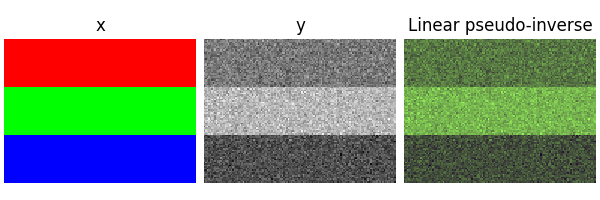
We test our physics on a toy image with 3 color channels. We add a Gaussian noise model to the linear physics.

We simulate measurements using the forward operator \(y=\forw{x}+\epsilon\). We then leverage the linear physics base class to automatically compute the linear pseudo-inverse \(A^\dagger y\).

x = torch.zeros(1, 3, 96, 128)
x[:, 0, :32, :] = 1
x[:, 1, 32:64, :] = 1
x[:, 2, 64:, :] = 1

physics = Decolorize(
    img_size=(3, 96, 128), noise_model=dinv.physics.GaussianNoise(sigma=0.1)
)

y = physics(x)

dinv.utils.plot({"x": x, "y": y, "Linear pseudo-inverse": physics.A_dagger(y)})

It is often useful for reconstruction algorithms that the physics has unit norm, which you can verify using deepinv.physics.LinearPhysics.compute_norm(). We see that this physics fails this.

print(f"The linear operator has norm={physics.compute_norm(x):.2f}")

Power iteration converged at iteration 2, value=0.45
The linear operator has norm=0.45

All parameters or buffers of the physics, such as coefficients in the case of Decolorize, can be updated on the fly with physics.update(**params) or in the forward pass physics(x, **params):

print(
    "Original coefficients and sigma:", physics.coefficients, physics.noise_model.sigma
)

physics.update(coefficients=torch.tensor([1.0, 2.0, 3.0]), sigma=0.2)

print(
    "Updated coefficients and sigma via update:",
    physics.coefficients,
    physics.noise_model.sigma,
)

y = physics(x, coefficients=torch.tensor([4.0, 5.0, 6.0]), sigma=0.3)

print(
    "Updated coefficients and sigma via forward pass:",
    physics.coefficients,
    physics.noise_model.sigma,
)

Original coefficients and sigma: tensor([0.2989, 0.5870, 0.1140]) tensor(0.1000)
Updated coefficients and sigma via update: tensor([1., 2., 3.]) tensor(0.2000)
Updated coefficients and sigma via forward pass: tensor([4., 5., 6.]) tensor(0.3000)

Implementing a closed form adjoint

Instead, if we know the closed form of the adjoint operator, we can implement it directly in deepinv.physics.LinearPhysics.A_adjoint(), instead of relying on autodifferentiation which is generally less efficient.

An additional benefit of implementing the adjoint is that we no longer require the img_size parameter when creating the operator, which was needed for autodifferentiation.

If you implement your own adjoint, it is recommended to verify that it is well-defined using deepinv.physics.LinearPhysics.adjointness_test().

class Decolorize2(Decolorize):
    """Override previous Decolorize using a closed-form adjoint."""

    def A_adjoint(
        self, y: torch.Tensor, coefficients: torch.Tensor = None, **kwargs
    ) -> torch.Tensor:
        """Closed-form adjoint operator.

        :param torch.Tensor y: input grayscale measurements
        :param torch.Tensor coefficients: optionally set coefficients on the fly
        :param dict kwargs: any other keyword parameters to set on the fly, such as noise model sigma
        :return: torch.Tensor adjoint reconstruction
        """
        super().update_parameters(coefficients=coefficients, **kwargs)

        return y * self.coefficients[None, :, None, None]


physics = Decolorize2()

if physics.adjointness_test(x) < 1e-5:
    print("The linear operator has a well defined adjoint")

The linear operator has a well defined adjoint

Creating a decomposable forward operator.

If the forward operator has a closed form singular value decomposition (SVD), you should instead implement the operator using the deepinv.physics.DecomposablePhysics base class.

The operator \(A\) in this example has a known closed-form SVD:

\[A = U\text{diag}(s)V^{\top}\]

where \(\text{diag}(s)\) is the mask of singular values.

Tip

As in the case of LinearPhysics, V and U_adjoint are implemented using autodifferentiation by default, but you can implement them directly if you know the closed form of the operator.

class DecolorizeSVD(dinv.physics.DecomposablePhysics):
    r"""
    Converts RGB images to grayscale.

    We use unnormalized coefficients and a singular value of 0.447.

    Here, `U` and `U_adjoint` are set to the identity.
    """

    def __init__(self, **kwargs):
        super().__init__(mask=0.447, **kwargs)
        coefficients = torch.tensor([0.6687, 1.3132, 0.2550], dtype=torch.float32)
        self.register_buffer("coefficients", coefficients)

    def V_adjoint(self, x: torch.Tensor) -> torch.Tensor:
        y = x * self.coefficients[None, :, None, None]
        return torch.sum(y, dim=1, keepdim=True)

    def V(self, y: torch.Tensor) -> torch.Tensor:
        return y * self.coefficients[None, :, None, None]


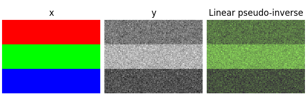
physics2 = DecolorizeSVD(noise_model=dinv.physics.GaussianNoise(sigma=0.1))

y2 = physics2(x)

dinv.utils.plot({"x": x, "y": y2, "Linear pseudo-inverse": physics2.A_dagger(y2)})

if physics.adjointness_test(x) < 1e-5:
    print("The decomposable operator has a well defined transpose")

print(f"The decomposable operator has norm={physics.compute_norm(x):.2f}")

The decomposable operator has a well defined transpose
Power iteration converged at iteration 2, value=0.45
The decomposable operator has norm=0.45

Benefits of using a decomposable forward operator.

The main benefit of using a decomposable forward operator is that it provides closed form solutions for the proximal operator and the linear pseudo-inverse. Moreover, some algorithms, such as deepinv.sampling.DDRM require the forward operator to be decomposable.

import time


def sync_cuda():
    if torch.cuda.is_available():
        torch.cuda.synchronize()


sync_cuda()
start = time.time()
for i in range(10):
    xlin = physics.A_dagger(y)
    xprox = physics.prox_l2(x, y, 0.1)

sync_cuda()
end = time.time()
print(f"Elapsed time for LinearPhysics: {end - start:.2f} seconds")

sync_cuda()
start = time.time()
for i in range(10):
    xlin2 = physics2.A_dagger(y)
    xprox2 = physics2.prox_l2(x, y2, 0.1)

sync_cuda()
end = time.time()
print(f"Elapsed time for DecomposablePhysics: {end - start:.2e} seconds")

Elapsed time for LinearPhysics: 0.01 seconds
Elapsed time for DecomposablePhysics: 2.07e-03 seconds

🎉 Well done, you now know how to implement your own physics!

What’s next?

• Check out the example on how to inference a state-of-the-art general pretrained model with your new physics.

• Check out the example on how to fine-tune a foundation model to your own physics.