Use iterative reconstruction algorithms

Follow this example to reconstruct images using an iterative algorithm.

The library provides a flexible framework to define your own iterative reconstruction algorithm, which are generally written as the optimization of the following problem:

\[\begin{equation} \label{eq:min_prob} \tag{1} \underset{x}{\arg\min} \quad \datafid{x}{y} + \lambda \reg{x}, \end{equation}\]

where \(\datafid{x}{y}\) is the data fidelity term, \(\reg{x}\) is the (explicit or implicit) regularization term, and \(\lambda\) is a regularization parameter. In this example, we demonstrate:

1. How to define your own iterative algorithm

2. How to package it as a reconstructor model

3. How to use predefined algorithms using optim builder

1. Defining your own iterative algorithm

import deepinv as dinv
import torch

device = dinv.utils.get_freer_gpu() if torch.cuda.is_available() else "cpu"

Define the physics of the problem

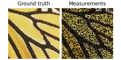
Here we define a simple inpainting problem, where we want to reconstruct an image from partial measurements. We also load an image of a butterfly to use as ground truth.

x = dinv.utils.load_example("butterfly.png", device=device, img_size=(128, 128))

# Forward operator, here inpainting with a mask of 50% of the pixels
physics = dinv.physics.Inpainting(img_size=(3, 128, 128), mask=0.5, device=device)

# Generate measurements
y = physics(x)

dinv.utils.plot([x, y], titles=["Ground truth", "Measurements"])

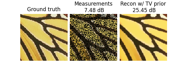
Define the data fidelity term and prior

The library provides a set of data fidelity terms and priors that can be used in the optimization problem. Here we use the \(\ell_2\) data fidelity term and the Total Variation (TV) prior.

These classes provide all the necessary methods for the optimization problem, such as the evaluation of the term, the gradient, and the proximal operator.

data_fidelity = dinv.optim.L2()  # Data fidelity term
prior = dinv.optim.TVPrior()  # Prior term

Define the iterative algorithm

We will use the Proximal Gradient Descent (PGD) algorithm to solve the optimization problem defined above, which is defined as

\[\qquad x_{k+1} = \operatorname{prox}_{\gamma \lambda \regname} \left( x_k - \gamma \nabla \datafidname(x_k, y) \right),\]

where \(\operatorname{prox}_{\gamma \lambda \regname}\) is the proximal operator of the regularization term, \(\nabla \datafidname(x_k, y)\) is the gradient of the data fidelity term, \(\gamma\) is the stepsize. and \(\lambda\) is the regularization parameter.

We can choose the stepsize as \(\gamma < \frac{2}{\|A\|^2}\), where \(A\) is the forward operator, in order to ensure convergence of the algorithm.

lambd = 0.05  # Regularization parameter

# Compute the squared norm of the operator A
norm_A2 = physics.compute_norm(y, tol=1e-4, verbose=False).item()
stepsize = 1.9 / norm_A2  # stepsize for the PGD algorithm

# PGD algorithm
max_iter = 20  # number of iterations
x_k = torch.zeros_like(x, device=device)  # initial guess

# To store the cost at each iteration:
cost_history = torch.zeros(max_iter, device=device)

with torch.no_grad():  # disable autodifferentiation
    for it in range(max_iter):
        u = x_k - stepsize * data_fidelity.grad(x_k, y, physics)  # Gradient step
        x_k = prior.prox(u, gamma=lambd * stepsize)  # Proximal step
        cost = data_fidelity(x_k, y, physics) + lambd * prior(x_k)  # Compute the cost
        cost_history[it] = cost  # Store the cost

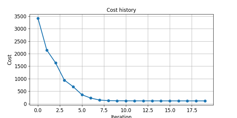
Plot the cost history

import matplotlib.pyplot as plt

plt.figure(figsize=(8, 4))
plt.plot(cost_history.detach().cpu().numpy(), marker="o")
plt.title("Cost history")
plt.xlabel("Iteration")
plt.ylabel("Cost")
plt.grid()
plt.show()

Plot the results and metrics

metric = dinv.metric.PSNR()

dinv.utils.plot(
    {
        f"Ground truth": x,
        f"Measurements\n {metric(y, x).item():.2f} dB": y,
        f"Recon w/ TV prior\n {metric(x_k, x).item():.2f} dB": x_k,
    }
)

Use a pretrained denoiser as prior

We can improve the reconstruction by using a pretrained denoiser as prior, by replacing the proximal operator with a denoising step. The library provides a collection of classical and pretrained denoisers that can be used in iterative algorithms.

Note

Plug-and-play algorithms can be sensitive to the choice of initialization. Here we use the TV estimate as the initial guess.

x_k = x_k.clone()

denoiser = dinv.models.DRUNet(device=device)  # Load a pretrained denoiser

with torch.no_grad():  # disable autodifferentiation
    for it in range(max_iter):
        u = x_k - stepsize * data_fidelity.grad(x_k, y, physics)  # Gradient step
        x_k = denoiser(u, sigma=0.05)  # replace prox by denoising step

dinv.utils.plot(
    {
        f"Ground truth": x,
        f"Measurements\n {metric(y, x).item():.2f} dB": y,
        f"Recon w/ PnP prior\n {metric(x_k, x).item():.2f} dB": x_k,
    }
)

2. Package your algorithm as a Reconstructor

The iterative algorithm we defined above can be packaged as a Reconstructor. This allows you to test it on different physics and datasets, and to use it in a more flexible way, including unfolding it and learning some of its parameters.

class MyPGD(dinv.models.Reconstructor):
    def __init__(self, data_fidelity, prior, stepsize, lambd, max_iter):
        super().__init__()
        self.data_fidelity = data_fidelity
        self.prior = prior
        self.stepsize = stepsize
        self.lambd = lambd
        self.max_iter = max_iter

    def forward(self, y, physics, **kwargs):
        """Algorithm forward pass.

        :param torch.Tensor y: measurements.
        :param dinv.physics.Physics physics: measurement operator.
        :return: torch.Tensor: reconstructed image.
        """
        x_k = torch.zeros_like(y, device=y.device)  # initial guess

        # Disable autodifferentiation, remove this if you want to unfold
        with torch.no_grad():
            for _ in range(self.max_iter):
                u = x_k - self.stepsize * self.data_fidelity.grad(
                    x_k, y, physics
                )  # Gradient step
                x_k = self.prior.prox(
                    u, gamma=self.lambd * self.stepsize
                )  # Proximal step

        return x_k


tv_algo = MyPGD(data_fidelity, prior, stepsize, lambd, max_iter)

# Standard reconstructor forward pass
x_hat = tv_algo(y, physics)

dinv.utils.plot(
    {
        f"Ground truth": x,
        f"Measurements\n {metric(y, x).item():.2f} dB": y,
        f"Recon w/ custom PGD\n {metric(x_hat, x).item():.2f} dB": x_hat,
    }
)

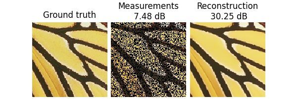
3. Using a predefined optimization algorithm with optim_builder

The library also lets you define standard optimization algorithms as standard Reconstructors in one line of code using the deepinv.optim.optim_builder function. For example, the above PnP algorithm can be defined as follows:

See also

See the optimization examples for more examples of using optim_builder.

prior = dinv.optim.PnP(denoiser=denoiser)  # prior with prox via denoising step


def custom_init(y: torch.Tensor, physics: dinv.physics.Physics) -> torch.Tensor:
    """
    Custom initialization function for the optimization algorithm.
    The function should return a dictionary with the key "est" containing a tuple
    with the initial guess (the TV solution in this case)
    and the dual variables (None in this case).
    """
    primal = tv_algo(y, physics)
    dual = None  #  No dual variables in this case
    return {"est": (primal, dual)}


model = dinv.optim.optim_builder(
    iteration="PGD",
    prior=prior,
    data_fidelity=data_fidelity,
    params_algo={"stepsize": stepsize, "g_param": 0.05},
    max_iter=max_iter,
    custom_init=custom_init,
)

x_hat = model(y, physics)

dinv.utils.plot(
    {
        f"Ground truth": x,
        f"Measurements\n {metric(y, x).item():.2f} dB": y,
        f"Reconstruction\n {metric(x_hat, x).item():.2f} dB": x_hat,
    }
)

🎉 Well done, you now know how to define your own iterative reconstruction algorithm!

What’s next?

• Check out more about optimization algorithms in the optimization user guide.

• Check out diffusion and MCMC iterative algorithms in the sampling user guide.

• Check out more iterative algorithms examples.

• Check out how to try the algorithm on a whole dataset by following the bring your own dataset tutorial.