Inference and fine-tune a foundation model

This example shows how to perform inference on and fine-tune the Reconstruct Anything Model (RAM) foundation model [1] to solve inverse problems.

The Reconstruct Anything Model is a model that has been trained to work on a large variety of linear image reconstruction tasks and datasets (deblurring, inpainting, denoising, tomography, MRI, etc.) and is robust to a wide variety of imaging domains.

Tip

• Want to use your own dataset? See Bring your own dataset

• Want to use your own physics? See Bring your own physics

import deepinv as dinv
import torch

device = dinv.utils.get_freer_gpu() if torch.cuda.is_available() else "cpu"

model = dinv.models.RAM(device=device, pretrained=True)

1. Zero-shot inference

First, let’s evaluate the zero-shot inference performance of the foundation model.

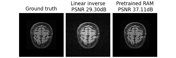
Accelerated medical imaging

Here, we demonstrated reconstructing brain MRI from an accelerated noisy MRI scan from FastMRI:

x = dinv.utils.load_example("demo_mini_subset_fastmri_brain_0.pt", device=device)

# Define physics
physics = dinv.physics.MRI(noise_model=dinv.physics.GaussianNoise(0.05), device=device)

physics_generator = dinv.physics.generator.GaussianMaskGenerator(
    (320, 320), device=device
)

# Generate measurement
y = physics(x, **physics_generator.step())

# Perform inference
with torch.no_grad():
    x_hat = model(y, physics)
    x_lin = physics.A_adjoint(y)

psnr = dinv.metric.PSNR()

dinv.utils.plot(
    {
        "Ground truth": x,
        f"Linear inverse": x_lin,
        f"Pretrained RAM": x_hat,
    },
    subtitles=[
        "PSNR:",
        f"{psnr(x, x_lin).item():.2f} dB",
        f"{psnr(x, x_hat).item():.2f} dB",
    ],
    figsize=(6, 4),
)

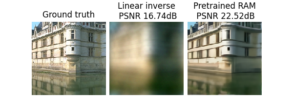
Computational photography

Joint random motion deblurring and denoising, using a cropped image from color BSD:

x = dinv.utils.load_example("CBSD_0010.png", img_size=(200, 200), device=device)

physics = dinv.physics.BlurFFT(
    img_size=x.shape[1:],
    noise_model=dinv.physics.GaussianNoise(sigma=0.05),
    device=device,
)

# fmt: off
physics_generator = (
    dinv.physics.generator.MotionBlurGenerator((31, 31), l=2.0, sigma=2.4, device=device) +
    dinv.physics.generator.SigmaGenerator(sigma_min=0.001, sigma_max=0.2, device=device)
)
# fmt: on

y = physics(x, **physics_generator.step())

with torch.no_grad():
    x_hat = model(y, physics)
    x_lin = physics.A_adjoint(y)

dinv.utils.plot(
    {
        "Ground truth": x,
        f"Linear inverse": x_lin,
        f"Pretrained RAM": x_hat,
    },
    subtitles=[
        "PSNR:",
        f"{psnr(x, x_lin).item():.2f} dB",
        f"{psnr(x, x_hat).item():.2f} dB",
    ],
    figsize=(6, 4),
)

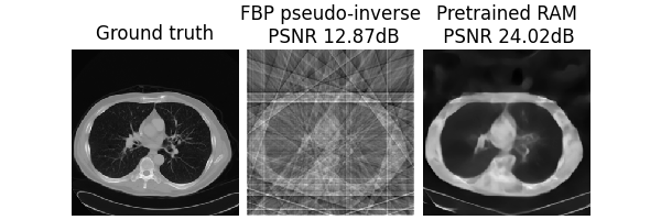
Tomography

Computed Tomography with limited angles using data from the The Cancer Imaging Archive of lungs:

x = dinv.utils.load_example("CT100_256x256_0.pt", device=device)

physics = dinv.physics.Tomography(
    img_width=256,
    angles=10,
    normalize=True,
    device=device,
)

y = physics(x)

with torch.no_grad():
    x_hat = model(y, physics)
    x_lin = physics.A_dagger(y)

dinv.utils.plot(
    {
        "Ground truth": x,
        f"FBP pseudo-inverse": x_lin,
        f"Pretrained RAM": x_hat,
    },
    subtitles=[
        "PSNR:",
        f"{psnr(x, x_lin).item():.2f} dB",
        f"{psnr(x, x_hat).item():.2f} dB",
    ],
    figsize=(6, 4),
)

Power iteration converged at iteration 8, ||A^T A||_2=2476.22

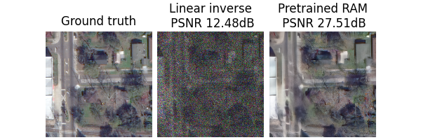
Remote sensing

Satellite denoising with Poisson-Gaussian noise using urban data from the WorldView-3 satellite over Jacksonville:

x = dinv.utils.load_example("JAX_018_011_RGB.tif", device=device)[..., :300, :300]

physics = dinv.physics.Denoising(
    noise_model=dinv.physics.PoissonGaussianNoise(sigma=0.1, gain=0.1)
)

y = physics(x)

with torch.no_grad():
    x_hat = model(y, physics)
    # Alternatively, use the model without physics:
    # x_hat = model(y, sigma=0.1, gain=0.1)
    x_lin = physics.A_adjoint(y)

dinv.utils.plot(
    {
        "Ground truth": x,
        f"Linear inverse": x_lin,
        f"Pretrained RAM": x_hat,
    },
    subtitles=[
        "PSNR:",
        f"{psnr(x, x_lin).item():.2f} dB",
        f"{psnr(x, x_hat).item():.2f} dB",
    ],
    figsize=(6, 4),
)

2. Fine-tuning

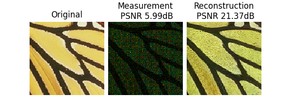
As with all models, there may be a drop in performance when used zero-shot on problems or data outside those seen during training.

For instance, RAM is not trained on image demosaicing:

x = dinv.utils.load_example("butterfly.png", img_size=(127, 129), device=device)

physics = dinv.physics.Demosaicing(
    img_size=x.shape[1:], noise_model=dinv.physics.PoissonNoise(0.1), device=device
)

# Generate measurement
y = physics(x)

# Run inference
with torch.no_grad():
    x_hat = model(y, physics)

# Show results
dinv.utils.plot(
    {
        "Original": x,
        f"Measurement": y,
        f"Reconstruction": x_hat,
    },
    subtitles=[
        "PSNR:",
        f"{psnr(x, y).item():.2f} dB",
        f"{psnr(x, x_hat).item():.2f} dB",
    ],
    figsize=(6, 4),
)

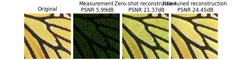
To improve results, we can fine-tune the model on our problem and data, even in the absence of ground truth data, using a self-supervised loss, and even on a single image only.

Here, since this example is run in a no-GPU environment, we will use a small patch of the image to speed up training, but in practice, we can use the full image.

Note

You can also fine-tune on larger datasets if you want, by replacing the dataset.

# Take small patch
x_train = x[..., :64, :64]

physics_train = dinv.physics.Demosaicing(
    img_size=x_train.shape[1:],
    noise_model=dinv.physics.PoissonNoise(0.1, clip_positive=True),
    device=device,
)

y_train = physics_train(x_train)

# Define training loss
losses = [
    dinv.loss.R2RLoss(),
    dinv.loss.EILoss(dinv.transform.Shift(shift_max=0.4), weight=0.1),
]

dataset = dinv.datasets.TensorDataset(y=y_train)
train_dataloader = torch.utils.data.DataLoader(dataset)

We fine-tune using early stopping on a validation set, again without ground truth. We use a small patch of another set of measurements as validation.

eval_dataloader = torch.utils.data.DataLoader(
    dinv.datasets.TensorDataset(
        y=physics_train(
            dinv.utils.load_example("leaves.png", device=device)[..., :64, :64]
        )
    )
)

max_epochs = 20
trainer = dinv.Trainer(
    model=model,
    physics=physics_train,
    eval_interval=5,
    ckp_interval=max_epochs - 1,
    metrics=None,
    compute_eval_losses=True,  # use self-supervised loss for evaluation
    early_stop_on_losses=True,  # stop using self-supervised eval loss
    early_stop=2,  # early stop after 2 evals without improvement
    device=device,
    losses=losses,
    epochs=max_epochs,
    optimizer=torch.optim.Adam(model.parameters(), lr=5e-5),
    train_dataloader=train_dataloader,
    eval_dataloader=eval_dataloader,
    show_progress_bar=False,  # disable progress bar for better vis in sphinx gallery.
)

finetuned_model = trainer.train()

finetuned_model = trainer.load_best_model()

The model has 35618953 trainable parameters
Train epoch 0: R2RLoss=0.126, EILoss=0.001, TotalLoss=0.128
Eval epoch 0: R2RLoss=0.143, EILoss=0.001, TotalLoss=0.144
Best model saved at epoch 1
Train epoch 1: R2RLoss=0.128, EILoss=0.0, TotalLoss=0.129
Train epoch 2: R2RLoss=0.129, EILoss=0.0, TotalLoss=0.129
Train epoch 3: R2RLoss=0.122, EILoss=0.0, TotalLoss=0.122
Train epoch 4: R2RLoss=0.131, EILoss=0.0, TotalLoss=0.132
Train epoch 5: R2RLoss=0.127, EILoss=0.0, TotalLoss=0.127
Eval epoch 5: R2RLoss=0.145, EILoss=0.001, TotalLoss=0.146
Train epoch 6: R2RLoss=0.128, EILoss=0.0, TotalLoss=0.128
Train epoch 7: R2RLoss=0.127, EILoss=0.0, TotalLoss=0.128
Train epoch 8: R2RLoss=0.123, EILoss=0.0, TotalLoss=0.123
Train epoch 9: R2RLoss=0.129, EILoss=0.0, TotalLoss=0.129
Train epoch 10: R2RLoss=0.125, EILoss=0.0, TotalLoss=0.125
Eval epoch 10: R2RLoss=0.153, EILoss=0.001, TotalLoss=0.153
Train epoch 11: R2RLoss=0.129, EILoss=0.0, TotalLoss=0.13
Train epoch 12: R2RLoss=0.129, EILoss=0.0, TotalLoss=0.13
Train epoch 13: R2RLoss=0.13, EILoss=0.0, TotalLoss=0.131
Train epoch 14: R2RLoss=0.125, EILoss=0.0, TotalLoss=0.125
Train epoch 15: R2RLoss=0.129, EILoss=0.0, TotalLoss=0.129
Eval epoch 15: R2RLoss=0.154, EILoss=0.001, TotalLoss=0.154
Early stopping triggered as validation metrics have not improved in the last 2 validation steps, disable it with early_stop=None, ormodify early_stop>0 to wait for more validation steps.

We can now use the fine-tuned model to reconstruct the image from the measurement y.

with torch.no_grad():
    x_hat_ft = finetuned_model(y, physics)

# Show results
dinv.utils.plot(
    {
        "Original": x,
        f"Measurement": y,
        f"Zero-shot \nReconstruction": x_hat,
        f"Fine-tuned \nReconstruction": x_hat_ft,
    },
    subtitles=[
        "PSNR:",
        f"{psnr(y, x).item():.2f} dB",
        f"{psnr(x, x_hat).item():.2f} dB",
        f"{psnr(x, x_hat_ft).item():.2f} dB",
    ],
    figsize=(6, 4),
)

References:

[1]

Matthieu Terris, Samuel Hurault, Maxime Song, and Julián Tachella. Reconstruct anything model: a lightweight foundation model for computational imaging. arXiv preprint arXiv:2503.08915, 2025.