BaseOptim#
- class deepinv.optim.BaseOptim(iterator, params_algo=MappingProxyType({'lambda': 1.0, 'stepsize': 1.0}), data_fidelity=None, prior=None, max_iter=100, crit_conv='residual', thres_conv=1e-5, early_stop=False, has_cost=False, backtracking=None, custom_metrics=None, custom_init=None, get_output=lambda X: ..., unfold=False, trainable_params=None, DEQ=None, anderson_acceleration=False, verbose=False, show_progress_bar=False, **kwargs)[source]#
Bases:
ReconstructorClass for optimization algorithms, consists in iterating a fixed-point operator.
Module solving the problem
\[\begin{equation} \label{eq:min_prob} \tag{1} \underset{x}{\arg\min} \quad \datafid{x}{y} + \lambda \reg{x}, \end{equation}\]where the first term \(\datafidname:\xset\times\yset \mapsto \mathbb{R}_{+}\) enforces data-fidelity, the second term \(\regname:\xset\mapsto \mathbb{R}_{+}\) acts as a regularization and \(\lambda > 0\) is a regularization parameter. More precisely, the data-fidelity term penalizes the discrepancy between the data \(y\) and the forward operator \(A\) applied to the variable \(x\), as
\[\datafid{x}{y} = \distance{Ax}{y}\]where \(\distance{\cdot}{\cdot}\) is a distance function, and where \(A:\xset\mapsto \yset\) is the forward operator (see
deepinv.physics.Physics)Optimization algorithms for minimising the problem above can be written as fixed point algorithms, i.e. for \(k=1,2,...\)
\[\qquad (x_{k+1}, z_{k+1}) = \operatorname{FixedPoint}(x_k, z_k, f, g, A, y, ...)\]where \(x_k\) is a variable converging to the solution of the minimization problem, and \(z_k\) is an additional “dual” variable that may be required in the computation of the fixed point operator.
If the algorithm is minimizing an explicit and fixed cost function \(F(x) = \datafid{x}{y} + \lambda \reg{x}\), the value of the cost function is computed along the iterations and can be used for convergence criterion. Moreover, backtracking can be used to adapt the stepsize at each iteration. Backtracking consists in choosing the largest stepsize \(\tau\) such that, at each iteration, sufficient decrease of the cost function \(F\) is achieved. More precisely, Given \(\gamma \in (0,1/2)\) and \(\eta \in (0,1)\) and an initial stepsize \(\tau > 0\), the following update rule is applied at each iteration \(k\):
\[\text{ while } F(x_k) - F(x_{k+1}) < \frac{\gamma}{\tau} || x_{k-1} - x_k ||^2, \,\, \text{ do } \tau \leftarrow \eta \tau\]Note
To use backtracking, the optimized function (i.e., both the the data-fidelity and prior) must be explicit and provide a computable cost for the current iterate. If the prior is not explicit (e.g. a denoiser) or if the argument
has_costis set toFalse, backtracking is automatically disabled.The variable
params_algois a dictionary containing all the relevant parameters for running the algorithm. If the value associated with the key is a float, the algorithm will use the same parameter across all iterations. If the value is list of length max_iter, the algorithm will use the corresponding parameter at each iteration.By default, the intial iterates are initialized with the adjoint applied to the measurement \(A^{\top}y\), when the adjoint is defined, and with the observation \(y\) if the adjoint is not defined. Custom initialization can be defined with the
custom_initclass argument or viainitargument in theforwardmethod.The variable
data_fidelityis a list of instances ofdeepinv.optim.DataFidelity(or a single instance). If a single instance, the same data-fidelity is used at each iteration. If a list, the data-fidelity can change at each iteration. The same holds for the variablepriorwhich is a list of instances ofdeepinv.optim.Prior(or a single instance).Setting
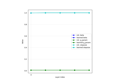
unfoldtoTrueenables to turn this iterative optimization algorithm into an unfolded algorithm, i.e. an algorithm that can be trained end-to-end, with learnable parameters. These learnable parameters encompass the trainable parameters of the algorithm which can be chosen with thetrainable_paramsargument (e.g.stepsize\(\gamma\), regularization parameterlambda_reg\(\lambda\), prior parameter (g_paramorsigma_denoiser) \(\sigma\) …) but also the trainable priors (e.g. a deep denoiser) or forward models.If
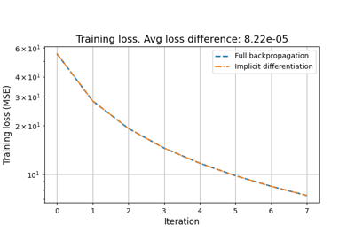
DEQis set toTrue, the algorithm is unfolded as a Deep Equilibrium model, i.e. the algorithm is virtually unrolled infinitely, leveraging the implicit function theorem. The backward pass is then performed using fixed point iterations to find solutions of the fixed-point equation\[\begin{equation} v = \left(\frac{\partial \operatorname{FixedPoint}(x^\star)}{\partial x^\star} \right )^{\top} v + u. \end{equation}\]where \(u\) is the incoming gradient from the backward pass, and \(x^\star\) is the equilibrium point of the forward pass. See this tutorial for more details.
Note also that by default, if the prior has trainable parameters (e.g. a neural network denoiser), these parameters are tranable by default.
Note
For now DEQ is only possible with PGD, HQS and GD optimization algorithms. If the model is used for inference only, use the
with torch.no_grad():context when calling the model in order to avoid unnecessary gradient computations.>>> import deepinv as dinv >>> # This minimal example shows how to use the BaseOptim class to solve the problem >>> # min_x 0.5 ||Ax-y||_2^2 + \lambda ||x||_1 >>> # with the PGD algorithm, where A is the identity operator, lambda = 1 and y = [2, 2]. >>> >>> # Create the measurement operator A >>> A = torch.tensor([[1, 0], [0, 1]], dtype=torch.float64) >>> A_forward = lambda v: A @ v >>> A_adjoint = lambda v: A.transpose(0, 1) @ v >>> >>> # Define the physics model associated to this operator >>> physics = dinv.physics.LinearPhysics(A=A_forward, A_adjoint=A_adjoint) >>> >>> # Define the measurement y >>> y = torch.tensor([2, 2], dtype=torch.float64) >>> >>> # Define the data fidelity term >>> data_fidelity = dinv.optim.data_fidelity.L2() >>> >>> # Define the prior >>> prior = dinv.optim.Prior(g = lambda x, *args: torch.linalg.vector_norm(x, ord=1, dim=tuple(range(1, x.ndim)))) >>> >>> # Define the parameters of the algorithm >>> params_algo = {"stepsize": 0.5, "lambda": 1.0} >>> >>> # Define the fixed-point iterator >>> iterator = dinv.optim.optim_iterators.PGDIteration() >>> >>> # Define the optimization algorithm >>> optimalgo = dinv.optim.BaseOptim(iterator, ... data_fidelity=data_fidelity, ... params_algo=params_algo, ... prior=prior) >>> >>> # Run the optimization algorithm >>> with torch.no_grad(): xhat = optimalgo(y, physics) >>> print(xhat) tensor([1., 1.], dtype=torch.float64)
- Parameters:
iterator (deepinv.optim.OptimIterator) – Fixed-point iterator of the optimization algorithm of interest.
params_algo (dict) – dictionary containing all the relevant parameters for running the algorithm, e.g. the stepsize, regularization parameter, denoising standard deviation. Each value of the dictionary can be either Iterable (distinct value for each iteration) or a single float (same value for each iteration). Default:
{"stepsize": 1.0, "lambda": 1.0}. See Optimization Parameters for more details.data_fidelity (deepinv.optim.DataFidelity, list[deepinv.optim.DataFidelity]) – data-fidelity term. Either a single instance (same data-fidelity for each iteration) or a list of instances of
deepinv.optim.DataFidelity(distinct data fidelity for each iteration). Default:Nonecorresponding to \(\datafid{x}{y} = 0\).prior (deepinv.optim.Prior, list[deepinv.optim.Prior]) – regularization prior. Either a single instance (same prior for each iteration) or a list of instances of
deepinv.optim.Prior(distinct prior for each iteration). Default:Nonecorresponding to \(\reg{x} = 0\).max_iter (int) – maximum number of iterations of the optimization algorithm. Default: 100.
crit_conv (str) – convergence criterion to be used for claiming convergence, either
"residual"(residual of the iterate norm) or"cost"(on the cost function). Default:"residual"thres_conv (float) – value of the threshold for claiming convergence. Default:
1e-05.early_stop (bool) – whether to stop the algorithm once the convergence criterion is reached. Default:
True.has_cost (bool) – whether the algorithm has an explicit cost function or not. Default:
False. If the prior is not explicit (e.g. a denoiser)prior.explicit_prior = False, thenhas_costis automatically set toFalse.custom_metrics (dict[str, deepinv.loss.metric.Metric]) – dictionary containing custom metrics to be computed at each iteration.
backtracking (BacktrackingConfig, bool) – configuration for using a backtracking line-search strategy for automatic stepsize adaptation. If
None(default) orFalse, stepsize backtracking is disabled. Otherwise,backtrackingmust be an instance ofdeepinv.optim.BacktrackingConfig, which defines the parameters for backtracking line-search. IfTrue, the defaultBacktrackingConfigis used.custom_init (Callable) –
Custom initialization of the algorithm. The callable function
custom_init(y, physics)takes as input the measurement \(y\) and the physicsphysicsand returns the initialization in the form of either:a tuple \((x_0, z_0)\) (where
x_0andz_0are the initial primal and dual variables),a torch.Tensor \(x_0\) (if no dual variables \(z_0\) are used), or
a dictionary of the form
X = {'est': (x_0, z_0)}.
Note that custom initialization can also be directly defined via the
initargument in theforwardmethod.If
None(default value), the algorithm is initialized with the adjoint \(A^{\top}y\) when the adjoint is defined, and with the observationyif the adjoint is not defined. Default:None.get_output (Callable) – Custom output of the algorithm. The callable function
get_output(X)takes as input the dictionaryXcontaining the primal and auxiliary variables and returns the desired output. Default :X['est'][0].unfold (bool) – whether to unfold the algorithm and make the model parameters trainable. Default:
False.trainable_params (list[str]) – list of the algorithmic parameters to be made trainable (must be chosen among the keys of the dictionary
params_algo). Default:None, which means that all parameters in params_algo are trainable. For no trainable parameters, set to an empty list[].DEQ (DEQConfig, bool) – Configuration for a Deep Equilibrium (DEQ) unfolding strategy. DEQ algorithms are virtually unrolled infinitely, leveraging the implicit function theorem. If
None(default) orFalse, DEQ is disabled and the algorithm runs a standard finite number of iterations. Otherwise,DEQmust be an instance ofdeepinv.optim.DEQConfig, which defines the parameters for forward and backward equilibrium-based implicit differentiation. IfTrue, the defaultDEQConfigis used.anderson_acceleration (AndersonAccelerationConfig, bool) – Configuration of Anderson acceleration for the fixed-point iterations. If
None(default) orFalse, Anderson acceleration is disabled. Otherwise,anderson_accelerationmust be an instance ofdeepinv.optim.AndersonAccelerationConfig, which defines the parameters for Anderson acceleration. IfTrue, the defaultAndersonAccelerationConfigis used.verbose (bool) – whether to print relevant information of the algorithm during its run, such as convergence criterion at each iterate. Default:
False.show_progress_bar (bool) – show progress bar during optimization.
- Returns:
a torch model that solves the optimization problem.
- DEQ_additional_step(X, y, physics, **kwargs)[source]#
For Deep Equilibrium models, performs an additional step at the equilibrium point to compute the gradient of the fixed point operator with respect to the input.
- Parameters:
X (dict) – dictionary defining the current update at the equilibrium point.
y (torch.Tensor) – measurement vector.
physics (deepinv.physics.Physics) – physics of the problem for the acquisition of
y.
- backtracking_check_fn(X_prev, X)[source]#
Performs stepsize backtracking if the sufficient decrease condition is not verified.
- forward(y, physics, init=None, x_gt=None, compute_metrics=False, **kwargs)[source]#
Runs the fixed-point iteration algorithm for solving (1).
- Parameters:
y (torch.Tensor) – measurement vector.
physics (deepinv.physics.Physics) – physics of the problem for the acquisition of
y.init (Callable, torch.Tensor, tuple, dict) –
initialization of the algorithm. Default:
None. ifNone(and the classcustom_init``argument is ``None), the algorithm is initialized with the adjoint \(A^{\top}y\) when the adjoint is defined, and with the observationyif the adjoint is not defined.initcan be either a fixed initialization or a Callable function of the forminit(y, physics)that takes as input the measurement \(y\) and the physicsphysics. The output of the function or the fixed initialization can be either:a tuple \((x_0, z_0)\) (where
x_0andz_0are the initial primal and dual variables),a
torch.Tensor\(x_0\) (if no dual variables \(z_0\) are used), ora dictionary of the form
X = {'est': (x_0, z_0)}.
Note that custom initialization can also be defined via the
custom_initclass argument.x_gt (torch.Tensor) – (optional) ground truth image, for plotting the PSNR across optim iterations.
compute_metrics (bool) – whether to compute the metrics or not. Default:
False.kwargs – optional keyword arguments for the optimization iterator (see
deepinv.optim.OptimIterator)
- Returns:
If
compute_metricsisFalse, returns (torch.Tensor) the output of the algorithm. Else, returns (torch.Tensor, dict) the output of the algorithm and the metrics.
- init_iterate_fn(y, physics, init=None, cost_fn=None)[source]#
Initializes the iterate of the algorithm. The first iterate is stored in a dictionary of the form
X = {'est': (x_0, u_0), 'cost': F_0}where:estis a tuple containing the first primal and auxiliary iterates.costis the value of the cost function at the first iterate.
By default, the first (primal and dual) iterate of the algorithm is chosen as \(A^{\top}y\) when the adjoint is defined, and with the observation
yif the adjoint is not defined. A custom initialization is possible via thecustom_initclass argument or via theinitargument.- Parameters:
y (torch.Tensor) – measurement vector.
deepinv.physics – physics of the problem.
init (Callable, torch.Tensor, tuple, dict) –
initialization of the algorithm. Either a Callable function of the form
init(y, physics)or a fixed torch.Tensor initialization. The output of the function or the fixed initialization can be either:a tuple \((x_0, z_0)\) (where
x_0andz_0are the initial primal and dual variables),a
torch.Tensor\(x_0\) (if no dual variables \(z_0\) are used), ora dictionary of the form
X = {'est': (x_0, z_0)}.
cost_fn (Callable) – function that computes the cost function.
cost_fn(x, data_fidelity, prior, cur_params, y, physics)takes as input the current primal variable (torch.Tensor), the current data-fidelity (deepinv.optim.DataFidelity), the current prior (deepinv.optim.Prior), the current parameters (dict), and the measurement (torch.Tensor). Default:None.
- Returns:
a dictionary containing the first iterate of the algorithm.
- Return type:
- init_metrics_fn(X_init, x_gt=None)[source]#
Initializes the metrics.
Metrics are computed for each batch and for each iteration. They are represented by a list of list, and
metrics[metric_name][i,j]contains the metricmetric_namecomputed for batch i, at iteration j.- Parameters:
X_init (dict) – dictionary containing the primal and auxiliary initial iterates.
x_gt (torch.Tensor) – ground truth image, required for PSNR computation. Default:
None.
- Return dict:
A dictionary containing the metrics.
- Return type:
- update_data_fidelity_fn(it)[source]#
For each data_fidelity function in
data_fidelity, selects the data_fidelity value for iterationit(if this data_fidelity depends on the iteration number).- Parameters:
it (int) – iteration number.
- Returns:
the data_fidelity at iteration
it.- Return type:
- update_metrics_fn(metrics, X_prev, X, x_gt=None)[source]#
Function that compute all the metrics, across all batches, for the current iteration.
- Parameters:
metrics (dict) – dictionary containing the metrics. Each metric is computed for each batch.
X_prev (dict) – dictionary containing the primal and dual previous iterates.
X (dict) – dictionary containing the current primal and dual iterates.
x_gt (torch.Tensor) – ground truth image, required for PSNR computation. Default: None.
- Return dict:
a dictionary containing the updated metrics.
- Return type:
Examples using BaseOptim:#
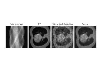
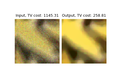
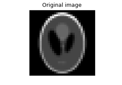
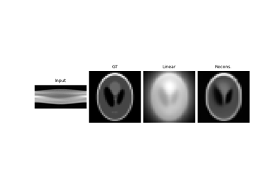
Low-dose CT with ASTRA backend and Total-Variation (TV) prior

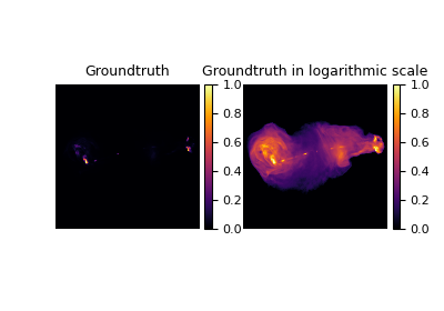
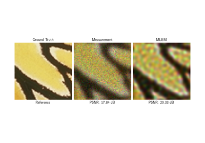
Poisson Inverse Problems with Maximum-Likelihood Expectation-Maximization (MLEM)

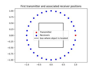
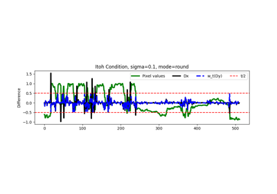
Random phase retrieval and reconstruction methods.
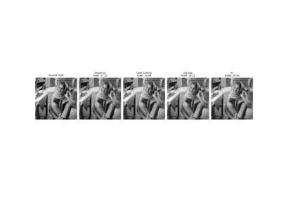
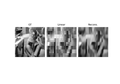
Pattern Ordering in a Compressive Single Pixel Camera
PnP with custom optimization algorithm (Primal-Dual Condat-Vu)
Plug-and-Play algorithm with Mirror Descent for Poisson noise inverse problems.
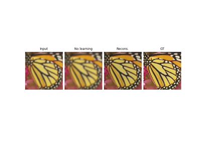
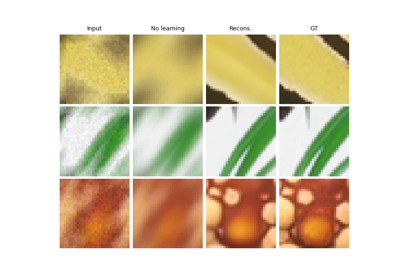
Regularization by Denoising (RED) for Super-Resolution.
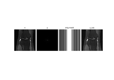
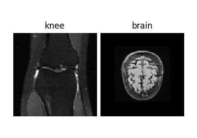
Self-supervised MRI reconstruction with Artifact2Artifact
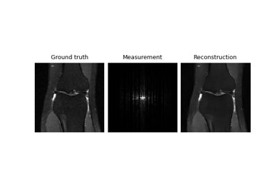
Self-supervised learning with Equivariant Imaging for MRI.
Deep Equilibrium (DEQ) algorithms for image deblurring
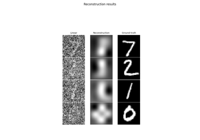
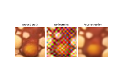
Learned Iterative Soft-Thresholding Algorithm (LISTA) for compressed sensing
Reducing the memory and computational complexity of unfolded network training

Unfolded Chambolle-Pock for constrained image inpainting