Blind deblurring with kernel estimation network

This example demonstrates blind image deblurring using the pretrained kernel estimation network from the paper Carbajal et al.[1]. The network estimates spatially-varying blur kernels from a blurred image, which are then used in a space-varying blur physics model to reconstruct the sharp image using a non-blind deblurring algorithm.

The model estimates 25 spatially-varying (33 x 33) blur kernels and corresponding spatial multipliers (weights) of the space-varying blur model:

\[y \approx \sum_{k=1}^{25} h_k \star (w_k \odot x)\]

where \(\star\) is a convolution, \(\odot\) is a Hadamard product, \(w_k\) are multipliers \(h_k\) are filters.

import torch
import deepinv as dinv
from deepinv.models import KernelIdentificationNetwork, RAM
from deepinv.optim import DPIR

device = dinv.utils.get_freer_gpu() if torch.cuda.is_available() else "cpu"

Selected GPU 0 with 5657.25 MiB free memory

Load blurry image

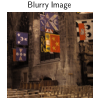
We load a real motion-blurred image from the Kohler dataset. You can access the whole dataset using deepinv.datasets.Kohler.

y = dinv.utils.load_example("kohler.png", device=device)[:, :3, ...]

dinv.utils.plot({"Blurry Image": y})  # plot blurry image

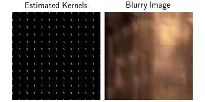
Estimate blur kernels

We use the pretrained kernel estimation network to estimate the spatially-varying blur kernels from the blurry image. The network provides 25 filters and corresponding spatial multipliers (weights) of the space-varying blur model (deepinv.physics.SpaceVaryingBlur).

We can visualise the estimated kernels by applying the forward operator to a Dirac comb input.

Note

The kernel estimation network is trained on non-gamma corrected images. If your input image is gamma-corrected (e.g., standard sRGB images), consider applying an inverse gamma correction before passing it to the network for better results.

# load pretrained kernel estimation network
kernel_estimator = KernelIdentificationNetwork(device=device)

# define space-varying blur physics
physics = dinv.physics.SpaceVaryingBlur(device=device, padding="constant")

with torch.no_grad():
    params = kernel_estimator(y)  # this outputs {"filters": ..., "multipliers": ...}
    physics.update(**params)
    dirac_comb = dinv.utils.dirac_comb_like(y, step=32)
    kernel_map = physics.A(dirac_comb)

    # visualize on a zoomed region
    dinv.utils.plot(
        {
            "Estimated Kernels": kernel_map[..., 128:512, 128:512],
            "Blurry Image": y[..., 200:300, 200:300],
        }
    )

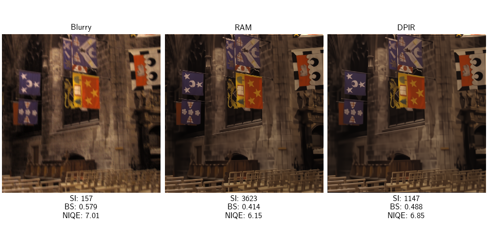
Deblur using non-blind reconstruction methods

Finally, we use two different non-blind deblurring algorithms to reconstruct the sharp image from the blurry observation and the estimated blur kernels: Here we use the general reconstruction model deepinv.models.RAM and the plug-and-play method deepinv.optim.DPIR.

model = RAM(device=device)
with torch.no_grad():
    x_ram = model(y, physics, sigma=0.05)
    x_ram = x_ram.clamp(0, 1)

model = DPIR(sigma=0.05, device=device)
x_dpir = model(y, physics)
x_dpir = x_dpir.clamp(0, 1)

No reference metrics and visualization

As here we assume that we do not have access to the ground truth sharp image, we cannot compute reference metrics such as PSNR or SSIM. However, we can still compute no-reference metrics such as NIQE (lower is better), Blur Strengh (lower is better) and Sharpness Index (higher is better) to assess the quality of the reconstructions.

center_crop = -10  # remove 10 pixels from each border to avoid boundary effects

niqe = dinv.metric.NIQE(center_crop=center_crop)

niqe_blurry = niqe(y).item()
niqe_ram = niqe(x_ram).item()
niqe_dpir = niqe(x_dpir).item()

bs = dinv.metric.BlurStrength(center_crop=center_crop)

bs_blurry = bs(y).item()
bs_ram = bs(x_ram).item()
bs_dpir = bs(x_dpir).item()

si = dinv.metric.SharpnessIndex(center_crop=center_crop)

si_blurry = si(y).item()
si_ram = si(x_ram).item()
si_dpir = si(x_dpir).item()


dinv.utils.plot(
    {"Blurry": y, "RAM": x_ram, "DPIR": x_dpir},
    subtitles=[
        f"SI: {si_blurry:.0f} \n BS: {bs_blurry:.3f} \n  NIQE: {niqe_blurry:.2f}",
        f"SI: {si_ram:.0f} \n BS: {bs_ram:.3f} \n  NIQE: {niqe_ram:.2f} ",
        f"SI: {si_dpir:.0f} \n BS: {bs_dpir:.3f} \n  NIQE: {niqe_dpir:.2f} ",
    ],
    figsize=(10, 5),
)

References:

[1]

Guillermo Carbajal, Patricia Vitoria, José Lezama, and Pablo Musé. Blind motion deblurring with pixel-wise kernel estimation via kernel prediction networks. IEEE Transactions on Computational Imaging, 9:928–943, 2023.