Single-pixel imaging with Spyrit

This example shows how to use Spyrit linear models and measurements with DeepInverse. Here we use the HadamSplit2d linear model from Spyrit.

Load images

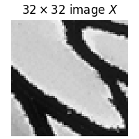
We start by loading the butterfly image using func:deepinv.utils.load_example:

import torch.nn

from deepinv.utils import plot
import deepinv as dinv

device = dinv.utils.get_freer_gpu() if torch.cuda.is_available() else "cpu"
im_size = 64
x = dinv.utils.load_example(
    "butterfly.png", device=device, img_size=(im_size, im_size), grayscale=True
)
print(f"Ground-truth image: {x.shape}")

Ground-truth image: torch.Size([1, 1, 64, 64])

Then we plot it:

plot(x, r"$32\times 32$ image $X$")

Basic example

We instantiate an HadamSplit2d object and simulate the 2D hadamard transform of the input images. Reshape output is necesary for deepinv. We also add Poisson noise.

from spyrit.core.meas import HadamSplit2d
from spyrit.core.prep import UnsplitRescale

physics_spyrit = HadamSplit2d(im_size, 512, device=device, reshape_output=True)
y_spyrit = physics_spyrit(x)

# preprocess
prep = UnsplitRescale(alpha=1.0)
y_spyrit = prep(y_spyrit)

print(y_spyrit.shape)

torch.Size([1, 1, 512])

The norm has to be computed to be passed to deepinv. We need to use the max singular value of the linear operator.

norm = torch.linalg.norm(physics_spyrit.H, ord=2)
print(norm)

tensor(64.0006)

Forward operator

You can direcly give the forward operator to deepinv. You can also add noise using deepinv model or spyrit model.

physics_deepinv = dinv.physics.LinearPhysics(
    lambda y: physics_spyrit.measure_H(y) / norm,
    A_adjoint=lambda y: physics_spyrit.unvectorize(physics_spyrit.adjoint_H(y) / norm),
)
y_deepinv = physics_deepinv(x)
print("diff:", torch.linalg.norm(y_spyrit / norm - y_deepinv))

diff: tensor(2.4486e-05)

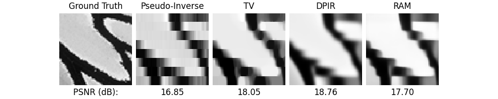
Computing the reconstructions

All of the usual solvers work out of the box and we showcase some of them here starting with simple linear reconstructions using deepinv.physics.LinearPhysics.A_adjoint() and deepinv.physics.LinearPhysics.A_dagger():

x_adj = physics_deepinv.A_adjoint(y_spyrit / norm)

x_pinv = physics_deepinv.A_dagger(y_spyrit / norm)

You can also use optimization-based methods from deepinv. Here, we use Total Variation (TV) regularization with a projected gradient descent (PGD) algorithm. You can note the use of the custom_init parameter to initialize the algorithm with the dagger operator.

model_tv = dinv.optim.optim_builder(
    iteration="PGD",
    prior=dinv.optim.TVPrior(),
    data_fidelity=dinv.optim.L2(),
    params_algo={"stepsize": 1, "lambda": 5e-2},
    max_iter=10,
    custom_init=lambda y, Physics: {"est": (Physics.A_dagger(y),)},
)

x_tv, metrics_TV = model_tv(
    y_spyrit / norm, physics_deepinv, compute_metrics=True, x_gt=x
)

And so do deep learning methods:

denoiser = dinv.models.DRUNet(in_channels=1, out_channels=1, device=device)
model_dpir = dinv.optim.DPIR(sigma=1e-1, device=device, denoiser=denoiser)
model_dpir.custom_init = lambda y, Physics: {"est": (Physics.A_dagger(y),)}
with torch.no_grad():
    x_dpir = model_dpir(y_spyrit / norm, physics_deepinv)

Including reconstruction with deepinv.models.RAM:

model_ram = dinv.models.RAM(pretrained=True, device=device)
model_ram.sigma_threshold = 1e-1
with torch.no_grad():
    x_ram = model_ram(y_spyrit / norm, physics_deepinv)

metric = dinv.metric.PSNR()

psnr_y = 0
psnr_pinv = metric(x_pinv, x).item()
psnr_tv = metric(x_tv, x).item()
psnr_dpir = metric(x_dpir, x).item()
psnr_ram = metric(x_ram, x).item()

dinv.utils.plot(
    {
        "Ground Truth": x,
        "Pseudo-Inverse": x_pinv,
        "TV": x_tv,
        "DPIR": x_dpir,
        "RAM": x_ram,
    },
    subtitles=[
        "PSNR (dB):",
        f"{psnr_pinv:.2f}",
        f"{psnr_tv:.2f}",
        f"{psnr_dpir:.2f}",
        f"{psnr_ram:.2f}",
    ],
)