Physics#
- class deepinv.physics.Physics(A=lambda x, **kwargs: ..., noise_model=None, sensor_model=lambda x: ..., solver='gradient_descent', max_iter=50, tol=1e-4, **kwargs)[source]#
Bases:
ModuleParent class for forward operators
It describes the general forward measurement process
\[y = \noise{\forw{x}}\]where \(x\) is an image of \(n\) pixels, \(y\) is the measurements of size \(m\), \(A:\xset\mapsto \yset\) is a deterministic mapping capturing the physics of the acquisition and \(N:\yset\mapsto \yset\) is a stochastic mapping which characterizes the noise affecting the measurements.
- Parameters:
A (Callable) – forward operator function which maps an image to the observed measurements \(x\mapsto y\).
noise_model (deepinv.physics.NoiseModel, Callable) – function that adds noise to the measurements \(\noise{z}\). See the noise module for some predefined functions.
sensor_model (Callable) – function that incorporates any sensor non-linearities to the sensing process, such as quantization or saturation, defined as a function \(\sensor{z}\), such that \(y=\sensor{\noise{\forw{x}}}\). By default, the
sensor_modelis set to the identity \(\sensor{z}=z\).max_iter (int) – If the operator does not have a closed form pseudoinverse, the gradient descent algorithm is used for computing it, and this parameter fixes the maximum number of gradient descent iterations.
tol (float) – If the operator does not have a closed form pseudoinverse, the gradient descent algorithm is used for computing it, and this parameter fixes the absolute tolerance of the gradient descent algorithm.
solver (str) – least squares solver to use. Only gradient descent is available for non-linear operators.
- A(x, **kwargs)[source]#
Computes forward operator \(y = A(x)\) (without noise and/or sensor non-linearities)
- Parameters:
x (torch.Tensor,list[torch.Tensor]) – signal/image
- Returns:
(
torch.Tensor) clean measurements
- A_dagger(y, x_init=None)[source]#
Computes an inverse as:
\[x^* \in \underset{x}{\arg\min} \quad \|\forw{x}-y\|^2.\]This function uses gradient descent to find the inverse. It can be overwritten by a more efficient pseudoinverse in cases where closed form formulas exist.
- Parameters:
y (torch.Tensor) – a measurement \(y\) to reconstruct via the pseudoinverse.
x_init (None, torch.Tensor) – initial guess for the reconstruction. If
None(default) it is set to the adjoint of the forward operator (it it exists) applied to the measurements \(y\), i.e., \(x_0 = A^{\top}y\).
- Returns:
(
torch.Tensor) The reconstructed image \(x\).
- A_vjp(x, v)[source]#
Computes the product between a vector \(v\) and the Jacobian of the forward operator \(A\) evaluated at \(x\), defined as:
\[A_{vjp}(x, v) = \left. \frac{\partial A}{\partial x} \right|_x^\top v.\]By default, the Jacobian is computed using automatic differentiation.
- Parameters:
x (torch.Tensor) – signal/image.
v (torch.Tensor) – vector.
- Returns:
(
torch.Tensor) the VJP product between \(v\) and the Jacobian.
- __mul__(other)[source]#
Concatenates two forward operators \(A = A_1\circ A_2\) via the mul operation
The resulting operator keeps the noise and sensor models of \(A_1\).
- Parameters:
other (deepinv.physics.Physics) – Physics operator \(A_2\)
- Returns:
(
deepinv.physics.Physics) concatenated operator
- clone()[source]#
Clone the forward operator by performing deepcopy to copy all attributes to new memory.
This method should be favored to
copy.deepcopyas it works even in the presence oftorch.Generatorobjects. Seethis issue <https://github.com/pytorch/pytorch/issues/43672>for more details.
- compute_norm(x, verbose=True)[source]#
Computes an estimate of the operator norm of the forward operator \(\|A\|_2\) at point
x.This function uses the power method to compute the operator norm.
- Parameters:
x (torch.Tensor) – input tensor used to estimate the norm.
verbose (bool) – if
True, prints the estimated norm.
- Returns:
(
torch.Tensor) estimated operator norm.
- forward(x, **kwargs)[source]#
Computes forward operator
\[y = N(A(x), \sigma)\]- Parameters:
x (torch.Tensor, list[torch.Tensor]) – signal/image
- Returns:
(
torch.Tensor) noisy measurements
- noise(x, **kwargs)[source]#
Incorporates noise into the measurements \(\tilde{y} = N(y)\)
- Parameters:
x (torch.Tensor) – clean measurements
noise_level (None, float) – optional noise level parameter
- Returns:
noisy measurements
- Return type:
- sensor(x)[source]#
Computes sensor non-linearities \(y = \eta(y)\)
- Parameters:
x (torch.Tensor,list[torch.Tensor]) – signal/image
- Returns:
(
torch.Tensor) clean measurements
- set_ls_solver(solver, max_iter=None, tol=None)[source]#
Change default solver for computing the least squares solution:
\[x^* \in \underset{x}{\arg\min} \quad \|\forw{x}-y\|^2.\]- Parameters:
solver (str) – solver to use. If the physics are non-linear, the only available solver is
'gradient_descent'. For linear operators, the options are'CG','lsqr','BiCGStab'and'minres'(seedeepinv.optim.linear.least_squares()for more details).max_iter (int) – maximum number of iterations for the solver.
tol (float) – relative tolerance for the solver, stopping when \(\|A(x) - y\| < \text{tol} \|y\|\).
- set_noise_model(noise_model, **kwargs)[source]#
Sets the noise model
- Parameters:
noise_model (Callable) – noise model
- stack(other)[source]#
Stacks two forward operators \(A(x) = \begin{bmatrix} A_1(x) \\ A_2(x) \end{bmatrix}\)
The measurements produced by the resulting model are
deepinv.utils.TensorListobjects, where each entry corresponds to the measurements of the corresponding operator.Returns a
deepinv.physics.StackedPhysicsobject.See Combining Physics for more information.
- Parameters:
other (deepinv.physics.Physics) – Physics operator \(A_2\)
- Returns:
(
deepinv.physics.StackedPhysics) stacked operator
Examples using Physics:#
Imaging inverse problems with adversarial networks
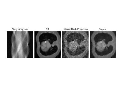
Low-dose CT with ASTRA backend and Total-Variation (TV) prior
Reconstructing an image using the deep image prior.
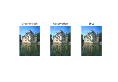
Expected Patch Log Likelihood (EPLL) for Denoising and Inpainting
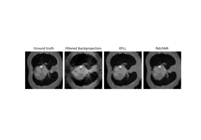
Patch priors for limited-angle computed tomography
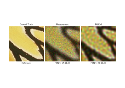
Poisson Inverse Problems with Maximum-Likelihood Expectation-Maximization (MLEM)
Random phase retrieval and reconstruction methods.
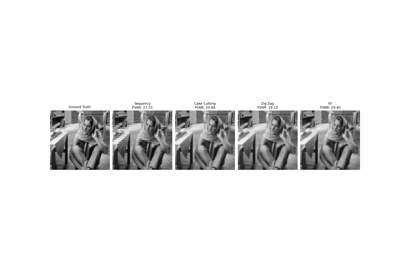
Pattern Ordering in a Compressive Single Pixel Camera
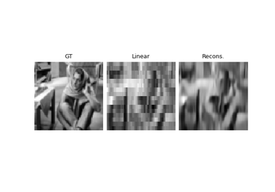
PnP with custom optimization algorithm (Primal-Dual Condat-Vu)
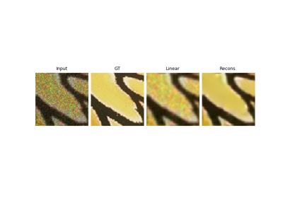
Plug-and-Play algorithm with Mirror Descent for Poisson noise inverse problems.
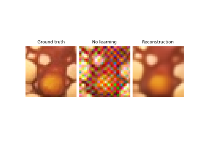
Regularization by Denoising (RED) for Super-Resolution.
Using state-of-the-art diffusion models from HuggingFace Diffusers with DeepInverse
Building your diffusion posterior sampling method using SDEs
Flow-Matching for posterior sampling and unconditional generation
Self-supervised MRI reconstruction with Artifact2Artifact
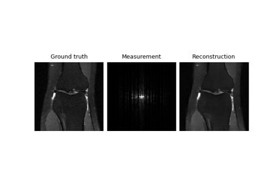
Self-supervised learning with Equivariant Imaging for MRI.
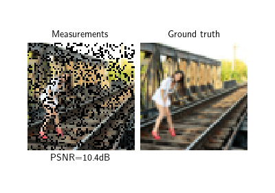
Self-supervised learning with Equivariant Splitting
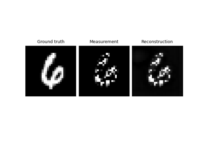
Self-supervised learning from incomplete measurements of multiple operators.
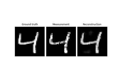
Self-supervised denoising with the Neighbor2Neighbor loss.
Self-supervised denoising with the Generalized R2R loss.
Self-supervised learning with measurement splitting
Deep Equilibrium (DEQ) algorithms for image deblurring
Learned Iterative Soft-Thresholding Algorithm (LISTA) for compressed sensing
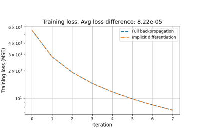
Reducing the memory and computational complexity of unfolded network training

Unfolded Chambolle-Pock for constrained image inpainting


