LinearPhysics#
- class deepinv.physics.LinearPhysics(A=lambda x, **kwargs: ..., A_adjoint=None, img_size=None, noise_model=ZeroNoise(), sensor_model=lambda x: ..., max_iter=50, tol=1e-4, solver='lsqr', implicit_backward_solver=True, device='cpu', **kwargs)[source]#
Bases:
PhysicsParent class for linear operators.
It describes the linear forward measurement process of the form
\[y = N(A(x))\]where \(x\) is an image of \(n\) pixels, \(y\) is the measurements of size \(m\), \(A:\xset\mapsto \yset\) is a deterministic linear mapping capturing the physics of the acquisition and \(N:\yset\mapsto \yset\) is a stochastic mapping which characterizes the noise affecting the measurements.
- Parameters:
A (Callable) – forward operator function which maps an image to the observed measurements \(x\mapsto y\). It is recommended to normalize it to have unit norm.
A_adjoint (None | Callable) – transpose of the forward operator, which should verify the adjointness test. By default, it is set to
None, which means that the adjoint is computed automatically usingdeepinv.physics.adjoint_function(). This automatic adjoint is computed using automatic differentiation, which is slower than a closed form adjoint, and can have a larger memory footprint. If you want to use the automatic adjoint, you should set theimg_sizeparameter If you have a closed form for the adjoint, you can pass it as a callable function or rewrite the class method.img_size (tuple) – (optional, only required if A_adjoint is not provided) Size of the signal/image
x, e.g.(C, ...)whereCis the number of channels and...are the spatial dimensions, used for the automatic adjoint computation.noise_model (Callable) – function that adds noise to the measurements \(N(z)\). See the noise module for some predefined functions.
sensor_model (Callable) – function that incorporates any sensor non-linearities to the sensing process, such as quantization or saturation, defined as a function \(\eta(z)\), such that \(y=\eta\left(N(A(x))\right)\). By default, the sensor_model is set to the identity \(\eta(z)=z\).
max_iter (int) – If the operator does not have a closed form pseudoinverse, the conjugate gradient algorithm is used for computing it, and this parameter fixes the maximum number of conjugate gradient iterations.
tol (float) – If the operator does not have a closed form pseudoinverse, a least squares algorithm is used for computing it, and this parameter fixes the relative tolerance of the least squares algorithm.
solver (str) – least squares solver to use. Choose between
'CG','lsqr','BiCGStab'and'minres'. Seedeepinv.optim.linear.least_squares()for more details.implicit_backward_solver (bool) – If
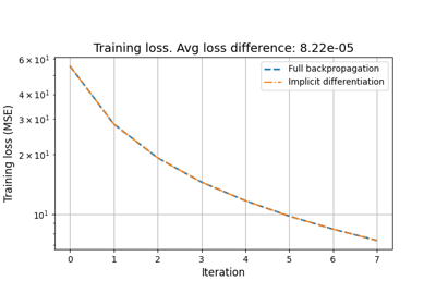
True, uses implicit differentiation for computing gradients through thedeepinv.physics.LinearPhysics.A_dagger()anddeepinv.physics.LinearPhysics.prox_l2(), usingdeepinv.optim.linear.least_squares_implicit_backward()instead ofdeepinv.optim.linear.least_squares(). This can significantly reduce memory consumption, especially when using many iterations. IfFalse, uses the standard autograd mechanism, which can be memory-intensive. Default isTrue.device (torch.device, str) – cpu or cuda, every registered buffer and module parameters are recursively pushed onto the device during initialization.
- Examples:
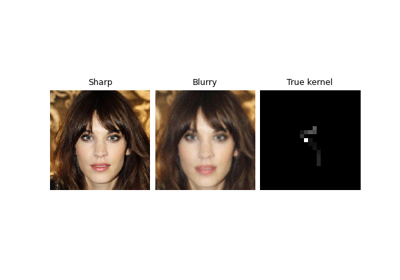
Blur operator with a basic averaging filter applied to a 32x32 black image with a single white pixel in the center:
>>> from deepinv.physics.blur import Blur, Downsampling
>>> x = torch.zeros((1, 1, 32, 32)) # Define black image of size 32x32
>>> x[:, :, 16, 16] = 1 # Define one white pixel in the middle
>>> w = torch.ones((1, 1, 3, 3)) / 9 # Basic 3x3 averaging filter
>>> physics = Blur(filter=w)
>>> y = physics(x)
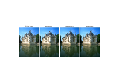
Linear operators can also be stacked. The measurements produced by the resulting model are
deepinv.utils.TensorListobjects, where each entry corresponds to the measurements of the corresponding operator (see Combining Physics for more information):>>> physics1 = Blur(filter=w) >>> physics2 = Downsampling(img_size=((1, 32, 32)), filter="gaussian", factor=4) >>> physics = physics1.stack(physics2) >>> y = physics(x)
Linear operators can also be composed by multiplying them:
>>> physics = physics1 * physics2
>>> y = physics(x)
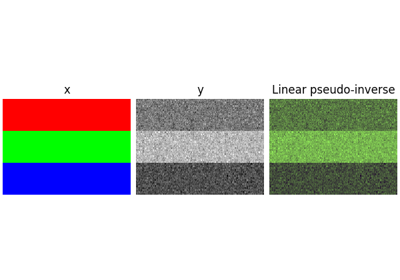
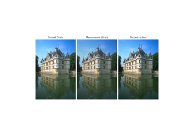
Linear operators also come with an adjoint, a pseudoinverse, and proximal operators in a given norm:
>>> from deepinv.loss.metric import PSNR
>>> physics = Blur(filter=w, padding='circular')
>>> y = physics(x) # Compute measurements
>>> x_dagger = physics.A_dagger(y) # Compute linear pseudoinverse
>>> x_prox = physics.prox_l2(torch.zeros_like(x), y, 1.) # Compute prox at x=0
>>> PSNR()(x, x_prox) > PSNR()(x, y) # Should be closer to the original
tensor([True])
The adjoint can be generated automatically using the
deepinv.physics.adjoint_function()method which relies on automatic differentiation, at the cost of a few extra computations per adjoint call:>>> from deepinv.physics import LinearPhysics, adjoint_function >>> A = lambda x: torch.roll(x, shifts=(1,1), dims=(2,3)) # Shift image by one pixel >>> physics = LinearPhysics(A=A, A_adjoint=adjoint_function(A, (4, 1, 5, 5))) >>> x = torch.randn((4, 1, 5, 5)) >>> y = physics(x) >>> torch.allclose(physics.A_adjoint(y), x) # We have A^T(A(x)) = x True
- A_A_adjoint(y, **kwargs)[source]#
A helper function that computes \(A A^{\top}y\).
This function can speed up computation when \(A A^{\top}\) is available in closed form. Otherwise it just calls
deepinv.physics.Physics.A()anddeepinv.physics.LinearPhysics.A_adjoint().- Parameters:
y (torch.Tensor) – measurement.
- Returns:
(
torch.Tensor) the product \(AA^{\top}y\).
- A_adjoint(y, **kwargs)[source]#
Computes transpose of the forward operator \(\tilde{x} = A^{\top}y\). If \(A\) is linear, it should be the exact transpose of the forward matrix.
Note
If the problem is non-linear, there is not a well-defined transpose operation, but defining one can be useful for some reconstruction networks, such as
deepinv.models.ArtifactRemoval.- Parameters:
y (torch.Tensor) – measurements.
params (None, torch.Tensor) – optional additional parameters for the adjoint operator.
- Returns:
(
torch.Tensor) linear reconstruction \(\tilde{x} = A^{\top}y\).
- A_adjoint_A(x, **kwargs)[source]#
A helper function that computes \(A^{\top}Ax\).
This function can speed up computation when \(A^{\top}A\) is available in closed form. Otherwise it just cals
deepinv.physics.Physics.A()anddeepinv.physics.LinearPhysics.A_adjoint().- Parameters:
x (torch.Tensor) – signal/image.
- Returns:
(
torch.Tensor) the product \(A^{\top}Ax\).
- A_dagger(y, solver='CG', max_iter=None, tol=None, verbose=False, **kwargs)[source]#
Computes the solution in \(x\) to \(y = Ax\) using a least squares solver.
This function can be overwritten by a more efficient pseudoinverse in cases where closed form formulas exist.
- Parameters:
y (torch.Tensor) – a measurement \(y\) to reconstruct via the pseudoinverse.
solver (str) – least squares solver to use. Choose between
'CG','lsqr','BiCGStab'and'minres'. Seedeepinv.optim.linear.least_squares()for more details.
- Returns:
(
torch.Tensor) The reconstructed image \(x\).
- A_vjp(x, v)[source]#
Computes the product between a vector \(v\) and the Jacobian of the forward operator \(A\) evaluated at \(x\), defined as:
\[A_{vjp}(x, v) = \left. \frac{\partial A}{\partial x} \right|_x^\top v = \conj{A} v.\]- Parameters:
x (torch.Tensor) – signal/image.
v (torch.Tensor) – vector of the size of the measurements.
- Returns:
(
torch.Tensor) the VJP product between \(v\) and the Jacobian.
- __mul__(other, **kwargs)[source]#
Concatenates two linear forward operators \(A = A_1 \circ A_2\) via the * operation
The resulting linear operator keeps the noise and sensor models of \(A_1\).
- Parameters:
other (deepinv.physics.LinearPhysics) – Physics operator \(A_2\)
- Returns:
(
deepinv.physics.LinearPhysics) concatenated operator
- adjointness_test(u, **kwargs)[source]#
Numerically check that \(A^{\top}\) is indeed the adjoint of \(A\).
- Parameters:
u (torch.Tensor) – initialization point of the adjointness test method
- Returns:
(float) a quantity that should be theoretically 0. In practice, it should be of the order of the chosen dtype precision (i.e. single or double).
- compute_norm(x0, max_iter=100, tol=1e-3, verbose=True, squared=True, **kwargs)[source]#
Computes the spectral \(\ell_2\) norm (Lipschitz constant) of the operator \(A\).
Warning
By default, for backward compatibility, this method computes the squared spectral norm of \(A\), i.e., \(\|A^{\top}A\|_2\). This behavior is deprecated and will change in a future version. Set
squared=Falseto compute the non-squared spectral norm \(\|A\|_2\), or usecompute_sqnorm()to explicitly compute the squared norm.Uses the power method.
- Parameters:
x0 (torch.Tensor) – an unbatched tensor sharing its shape, dtype and device with the initial iterate of the algorithm (its values are ignored)
max_iter (int) – maximum number of iterations
tol (float) – relative variation criterion for convergence
verbose (bool) – print information
squared (bool) – If
True(default, deprecated), computes \(\|A^{\top}A\|_2\) (squared spectral norm of \(A\)). Usecompute_sqnorm()instead. IfFalse, computes \(\|A\|_2\) (spectral norm of \(A\)).kwargs (dict) – optional parameters for the forward operator
- Returns:
(torch.Tensor) spectral norm. If
squared=True, returns \(\|A^{\top}A\|_2\) (squared spectral norm of \(A\)). Ifsquared=False, returns \(\|A\|_2\) (spectral norm of \(A\)).- Return type:
- compute_sqnorm(x0, *, max_iter=100, tol=1e-3, verbose=True, rng=None, **kwargs)[source]#
Computes the squared spectral \(\ell_2\) norm of the operator \(A\).
This is equivalent to computing the spectral norm of \(A^{\top}A\), i.e., \(\|A^{\top}A\|_2\).
Uses the power method.
- Parameters:
x0 (torch.Tensor) – an unbatched tensor sharing its shape, dtype and device with the initial iterate of the algorithm (its values are ignored)
max_iter (int) – maximum number of iterations
tol (float) – relative variation criterion for convergence
verbose (bool) – print information
kwargs (dict) – optional parameters for the forward operator
- Returns:
(torch.Tensor) squared spectral norm of \(A\), i.e., \(\|A^{\top}A\|_2 = \|A\|_2^2\).
- Return type:
- condition_number(x, max_iter=500, tol=1e-6, verbose=False, **kwargs)[source]#
Computes an approximation of the condition number of the linear operator \(A\).
Uses the LSQR algorithm, see
deepinv.optim.linear.lsqr()for more details.- Parameters:
x (torch.Tensor) – Any input tensor (e.g. random)
max_iter (int) – maximum number of iterations
tol (float) – relative variation criterion for convergence
verbose (bool) – print information
- Returns:
(
torch.Tensor) condition number of the operator
- property device: device | str#
Returns the device where the physics parameters/buffers are stored.
- Returns:
device of the physics parameters.
- prox_l2(z, y, gamma, solver='CG', max_iter=None, tol=None, verbose=False, **kwargs)[source]#
Computes proximal operator of \(f(x) = \frac{1}{2}\|Ax-y\|^2\), i.e.,
\[\underset{x}{\arg\min} \; \frac{\gamma}{2}\|Ax-y\|^2 + \frac{1}{2}\|x-z\|^2\]- Parameters:
y (torch.Tensor) – measurements tensor
z (torch.Tensor, float, int, None) – signal tensor
gamma (float) – hyperparameter of the proximal operator
solver (str) – solver to use for the proximal operator, see
deepinv.optim.linear.least_squares()for detailsmax_iter (int) – maximum number of iterations for iterative solvers
tol (float) – tolerance for iterative solvers
verbose (bool) – whether to print information during the solver execution
scale (int) – scale at which to apply the physics operator
- Returns:
(
torch.Tensor) estimated signal tensor
- stack(other)[source]#
Stacks forward operators \(A = \begin{bmatrix} A_1 \\ A_2 \end{bmatrix}\).
The measurements produced by the resulting model are
deepinv.utils.TensorListobjects, where each entry corresponds to the measurements of the corresponding operator.Note
When using the
stackoperator between two noise objects, the operation will retain only the second noise.See Combining Physics for more information.
- Parameters:
other (deepinv.physics.Physics) – Physics operator \(A_2\)
- Returns:
(
deepinv.physics.StackedPhysics) stacked operator
Examples using LinearPhysics:#
Imaging inverse problems with adversarial networks
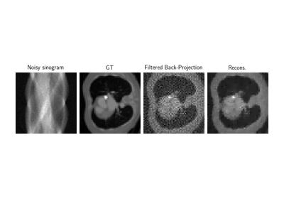
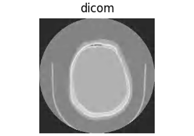
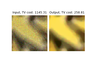
Low-dose CT with ASTRA backend and Total-Variation (TV) prior

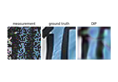
Reconstructing an image using the deep image prior.
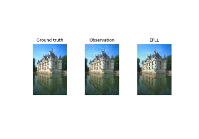
Expected Patch Log Likelihood (EPLL) for Denoising and Inpainting
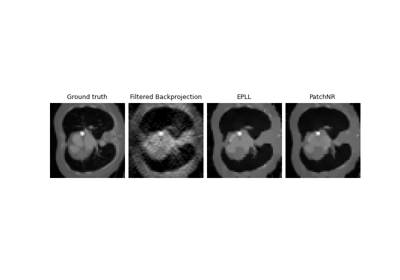
Patch priors for limited-angle computed tomography
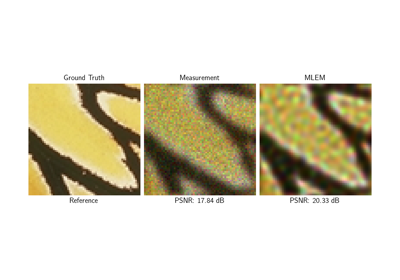
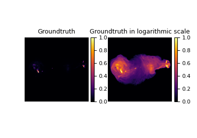
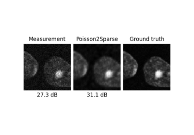
Poisson Inverse Problems with Maximum-Likelihood Expectation-Maximization (MLEM)

Poisson-Gaussian Denoising with the Generalized Anscombe Transform

Pattern Ordering in a Compressive Single Pixel Camera
PnP with custom optimization algorithm (Primal-Dual Condat-Vu)
Plug-and-Play algorithm with Mirror Descent for Poisson noise inverse problems.
Regularization by Denoising (RED) for Super-Resolution.
Using state-of-the-art diffusion models from HuggingFace Diffusers with DeepInverse
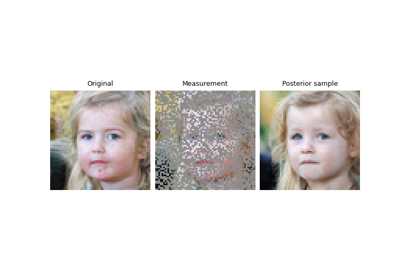
Building your diffusion posterior sampling method using SDEs

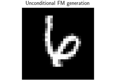
Flow-Matching for posterior sampling and unconditional generation

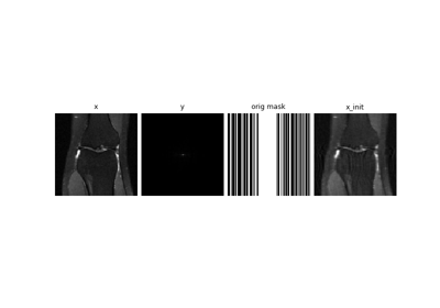
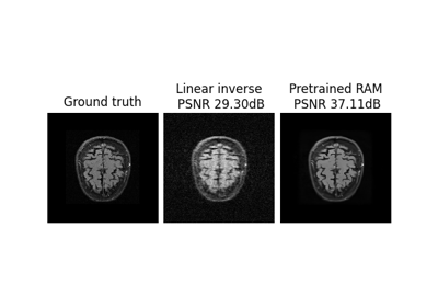
Self-supervised MRI reconstruction with Artifact2Artifact
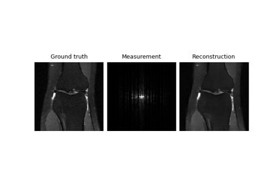
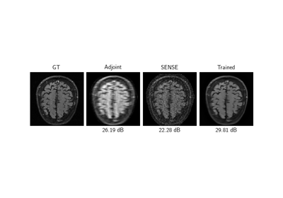
Self-supervised learning with Equivariant Imaging for MRI.
Self-supervised learning with Equivariant Splitting
Self-supervised learning from incomplete measurements of multiple operators.
Self-supervised denoising with the Neighbor2Neighbor loss.
Self-supervised denoising with the Generalized R2R loss.
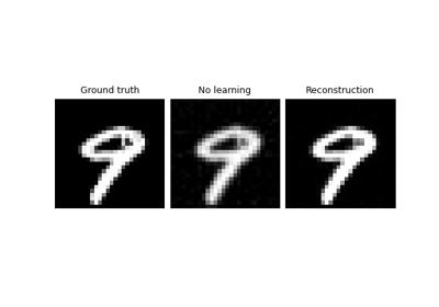
Self-supervised learning with measurement splitting

Deep Equilibrium (DEQ) algorithms for image deblurring
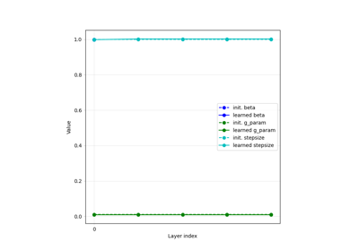
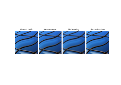
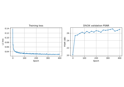
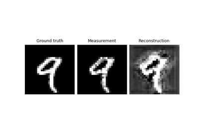
Learned Iterative Soft-Thresholding Algorithm (LISTA) for compressed sensing

Reducing the memory and computational complexity of unfolded network training

Unfolded Chambolle-Pock for constrained image inpainting