DataFidelity#
- class deepinv.optim.DataFidelity(d=None)[source]#
Bases:
PotentialBase class for the data fidelity term \(\distance{A(x)}{y}\) where \(A\) is the forward operator, \(x\in\xset\) is a variable and \(y\in\yset\) is the data, and where \(d\) is a distance function, from the class
deepinv.optim.Distance.- Parameters:
d (Callable) – distance function \(d(x, y)\) between a variable \(x\) and an observation \(y\). Default None.
- fn(x, y, physics, *args, **kwargs)[source]#
Computes the data fidelity term \(\datafid{x}{y} = \distance{\forw{x}}{y}\).
- Parameters:
x (torch.Tensor) – Variable \(x\) at which the data fidelity is computed.
y (torch.Tensor) – Data \(y\).
physics (deepinv.physics.Physics) – physics model.
- Returns:
(
torch.Tensor) data fidelity \(\datafid{x}{y}\).- Return type:
- grad(x, y, physics, *args, **kwargs)[source]#
Calculates the gradient of the data fidelity term \(\datafidname\) at \(x\).
The gradient is computed using the chain rule:
\[\nabla_x \distance{\forw{x}}{y} = \left. \frac{\partial A}{\partial x} \right|_x^\top \nabla_u \distance{u}{y},\]where \(\left. \frac{\partial A}{\partial x} \right|_x\) is the Jacobian of \(A\) at \(x\), and \(\nabla_u \distance{u}{y}\) is computed using
grad_dwith \(u = \forw{x}\). The multiplication is computed using theA_vjpmethod of the physics.- Parameters:
x (torch.Tensor) – Variable \(x\) at which the gradient is computed.
y (torch.Tensor) – Data \(y\).
physics (deepinv.physics.Physics) – physics model.
- Returns:
(
torch.Tensor) gradient \(\nabla_x \datafid{x}{y}\), computed in \(x\).- Return type:
- grad_d(u, y, *args, **kwargs)[source]#
Computes the gradient \(\nabla_u\distance{u}{y}\), computed in \(u\).
Note that this is the gradient of \(\distancename\) and not \(\datafidname\). This function directly calls
deepinv.optim.Potential.grad()for the specific distance function \(\distancename\).- Parameters:
u (torch.Tensor) – Variable \(u\) at which the gradient is computed.
y (torch.Tensor) – Data \(y\) of the same dimension as \(u\).
- Returns:
(
torch.Tensor) gradient of \(d\) in \(u\), i.e. \(\nabla_u\distance{u}{y}\).- Return type:
- prox_d(u, y, *args, **kwargs)[source]#
Computes the proximity operator \(\operatorname{prox}_{\gamma\distance{\cdot}{y}}(u)\), computed in \(u\).
Note that this is the proximity operator of \(\distancename\) and not \(\datafidname\). This function directly calls
deepinv.optim.Potential.prox()for the specific distance function \(\distancename\).- Parameters:
u (torch.Tensor) – Variable \(u\) at which the gradient is computed.
y (torch.Tensor) – Data \(y\) of the same dimension as \(u\).
- Returns:
(
torch.Tensor) gradient of \(d\) in \(u\), i.e. \(\nabla_u\distance{u}{y}\).- Return type:
- prox_d_conjugate(u, y, *args, **kwargs)[source]#
Computes the proximity operator of the convex conjugate of the distance function \(\distance{u}{y}\).
This function directly calls
deepinv.optim.Potential.prox_conjugate()for the specific distance function \(\distancename\).
Examples using DataFidelity:#
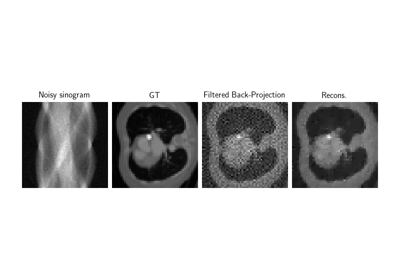
Low-dose CT with ASTRA backend and Total-Variation (TV) prior
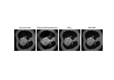
Patch priors for limited-angle computed tomography
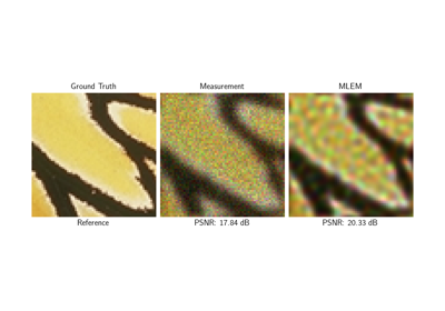
Poisson Inverse Problems with Maximum-Likelihood Expectation-Maximization (MLEM)
Random phase retrieval and reconstruction methods.
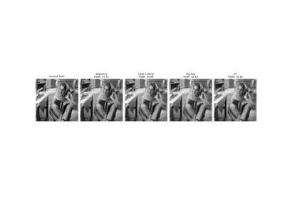
Pattern Ordering in a Compressive Single Pixel Camera
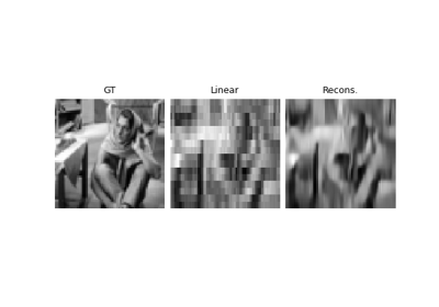
PnP with custom optimization algorithm (Primal-Dual Condat-Vu)
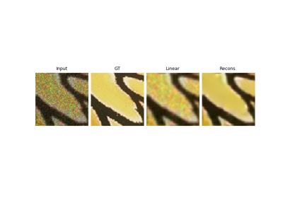
Plug-and-Play algorithm with Mirror Descent for Poisson noise inverse problems.
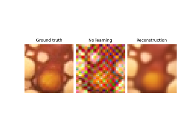
Regularization by Denoising (RED) for Super-Resolution.
Using state-of-the-art diffusion models from HuggingFace Diffusers with DeepInverse
Building your diffusion posterior sampling method using SDEs
Flow-Matching for posterior sampling and unconditional generation
Deep Equilibrium (DEQ) algorithms for image deblurring
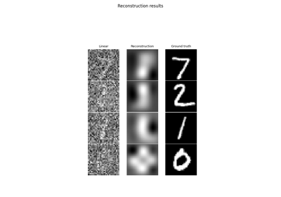
Learned Iterative Soft-Thresholding Algorithm (LISTA) for compressed sensing
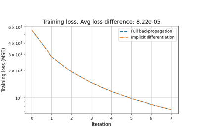
Reducing the memory and computational complexity of unfolded network training

Unfolded Chambolle-Pock for constrained image inpainting


