Distributed Physics Operators

Many large-scale imaging problems involve operators that can be naturally decomposed as a stack of multiple sub-operators:

\[\begin{split}A(x) = \begin{bmatrix} A_1(x) \\ \vdots \\ A_N(x) \end{bmatrix}\end{split}\]

where each sub-operator \(A_i\) is computationally expensive. Examples include multi-coil MRI, radio interferometry with multiple antennas, or multi-sensor imaging systems where each sensor provides a different measurement.

The distributed framework enables you to parallelize the computation of these operators across multiple devices. Each device handles a subset of the sub-operators independently, and the results are automatically assembled. This is particularly useful when the forward operator \(A\), its adjoint \(A^{\top}\), or composition \(A^{\top}A\) is computationally intensive.

This example demonstrates how to use deepinv.distributed.distribute() to distribute stacked physics operators across multiple processes/devices for parallel computation.

Usage:

# Single process
python examples/distributed/demo_physics_distributed.py

# Multi-process with torchrun (2 processes)
python -m torch.distributed.run --nproc_per_node=2 examples/distributed/demo_physics_distributed.py

Key Features:

• Distribute multiple operators across processes/devices

• Parallel forward operations \(A\)

• Parallel adjoint operations \(A^{\top}\)

• Parallel composition \(A^{\top} A\)

• Automatic result assembly from distributed processes

Key Steps:

1. Create multiple physics operators with different blur kernels

2. Stack them using deepinv.physics.stack()

3. Initialize distributed context

4. Distribute physics with deepinv.distributed.distribute()

5. Apply forward, adjoint, and composition operations

6. Visualize results

Import modules and define noisy image generation

We start by importing torch and the modules of deepinv that we use in this example. We also define a function that generates noisy images to evaluate the distributed framework.

import torch
from deepinv.physics import Blur, stack
from deepinv.physics.blur import gaussian_blur
from deepinv.utils.demo import load_example
from deepinv.utils.plotting import plot

# Import distributed framework
from deepinv.distributed import DistributedContext, distribute


def create_stacked_physics(device, img_size=1024):
    """
    Create stacked physics operators with different Gaussian blur kernels.

    :param device: Device to create operators on
    :param tuple img_size: Size of the image (H, W)
    :returns: Tuple of (stacked_physics, clean_image)
    """
    # Load example image
    clean_image = load_example(
        "CBSD_0010.png",
        grayscale=False,
        device=device,
        img_size=img_size,
        resize_mode="resize",
    )

    # Create different Gaussian blur kernels
    kernels = [
        gaussian_blur(sigma=1.0, device=str(device)),  # Small blur
        gaussian_blur(sigma=2.5, device=str(device)),  # Medium blur
        gaussian_blur(
            sigma=(1.5, 3.5), angle=30, device=str(device)
        ),  # Anisotropic blur
    ]

    # Create physics operators (without noise for exact comparison)
    physics_list = []

    for kernel in kernels:
        # Create blur operator with circular padding
        physics = Blur(filter=kernel, padding="circular", device=str(device))
        physics = physics.to(device)

        physics_list.append(physics)

    # Stack physics operators into a single operator
    stacked_physics = stack(*physics_list)

    return stacked_physics, clean_image

Configuration of parallel physics

img_size = 512

Define distributed context and run algorithm

# Initialize distributed context (handles single and multi-process automatically)
with DistributedContext(seed=42) as ctx:

    if ctx.rank == 0:
        print("=" * 70)
        print("Distributed Physics Operators Demo")
        print("=" * 70)
        print(f"\nRunning on {ctx.world_size} process(es)")
        print(f"   Device: {ctx.device}")

    # ---------------------------------------------------------------------------
    # Step 1: Create stacked physics operators
    # ---------------------------------------------------------------------------

    stacked_physics, clean_image = create_stacked_physics(ctx.device, img_size=img_size)

    if ctx.rank == 0:
        print(f"\nCreated stacked physics with {len(stacked_physics)} operators")
        print(f"   Image shape: {clean_image.shape}")
        print(
            f"   Operator types: {[type(p).__name__ for p in stacked_physics.physics_list]}"
        )

    # ---------------------------------------------------------------------------
    # Step 2: Distribute physics across processes
    # ---------------------------------------------------------------------------

    distributed_physics = distribute(stacked_physics, ctx)

    if ctx.rank == 0:
        print(f"\n Distributed physics created")
        print(
            f"   Local operators on this rank: {len(distributed_physics.local_indexes)}"
        )

    # ---------------------------------------------------------------------------
    # Step 3: Test forward operation (A)
    # ---------------------------------------------------------------------------

    if ctx.rank == 0:
        print(f"\n Testing forward operation (A)...")

    # Apply distributed forward operation
    measurements = distributed_physics(clean_image)

    # Compare with non-distributed result (only on rank 0)
    measurements_ref = None
    if ctx.rank == 0:
        print(f"   Output type: {type(measurements).__name__}")
        print(f"   Number of measurements: {len(measurements)}")
        for i, m in enumerate(measurements):
            print(f"   Measurement {i} shape: {m.shape}")

        print(f"\n Comparing with non-distributed forward operation...")
        measurements_ref = stacked_physics(clean_image)

        max_diff = 0.0
        mean_diff = 0.0
        for i in range(len(measurements)):
            diff = torch.abs(measurements[i] - measurements_ref[i])
            max_diff = max(max_diff, diff.max().item())
            mean_diff += diff.mean().item()
        mean_diff /= len(measurements)

        print(f"   Mean absolute difference: {mean_diff:.2e}")
        print(f"   Max absolute difference:  {max_diff:.2e}")

        # Assert exact equality (should be zero for deterministic operations)
        assert (
            max_diff < 1e-6
        ), f"Distributed forward operation differs from non-distributed: max diff = {max_diff}"
        print(f"   Results match exactly!")

    # ---------------------------------------------------------------------------
    # Step 4: Test adjoint operation (A^T)
    # ---------------------------------------------------------------------------

    if ctx.rank == 0:
        print(f"\nTesting adjoint operation (A^T)...")

    # Apply adjoint operation
    adjoint_result = distributed_physics.A_adjoint(measurements)

    if ctx.rank == 0:
        print(f"   Output shape: {adjoint_result.shape}")
        print(f"   Output norm: {torch.linalg.norm(adjoint_result).item():.4f}")

        # Compare with non-distributed result
        print(f"\nComparing with non-distributed adjoint operation...")
        assert measurements_ref is not None
        adjoint_ref = stacked_physics.A_adjoint(measurements_ref)
        diff = torch.abs(adjoint_result - adjoint_ref)
        print(f"   Mean absolute difference: {diff.mean().item():.2e}")
        print(f"   Max absolute difference:  {diff.max().item():.2e}")

        # Assert exact equality
        assert (
            diff.max().item() < 1e-6
        ), f"Distributed adjoint differs from non-distributed: max diff = {diff.max().item()}"
        print(f"   Results match exactly!")

    # ---------------------------------------------------------------------------
    # Step 5: Test composition (A^T A)
    # ---------------------------------------------------------------------------

    if ctx.rank == 0:
        print(f"\nTesting composition (A^T A)...")

    # Apply composition
    ata_result = distributed_physics.A_adjoint_A(clean_image)

    if ctx.rank == 0:
        print(f"   Output shape: {ata_result.shape}")
        print(f"   Output norm: {torch.linalg.norm(ata_result).item():.4f}")

        # Compare with non-distributed result
        print(f"\nComparing with non-distributed A^T A operation...")
        ata_ref = stacked_physics.A_adjoint_A(clean_image)
        diff = torch.abs(ata_result - ata_ref)
        print(f"   Mean absolute difference: {diff.mean().item():.2e}")
        print(f"   Max absolute difference:  {diff.max().item():.2e}")

        # Assert exact equality
        assert (
            diff.max().item() < 1e-6
        ), f"Distributed A^T A differs from non-distributed: max diff = {diff.max().item()}"
        print(f"   Results match exactly!")

    # ---------------------------------------------------------------------------
    # Step 6: Visualize results (only on rank 0)
    # ---------------------------------------------------------------------------

    if ctx.rank == 0:
        print(f"\nVisualizing results...")

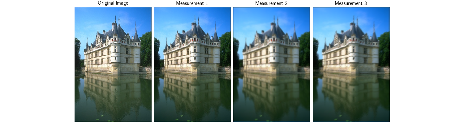
        # Plot original image and measurements
        images_to_plot = [clean_image] + [m for m in measurements]
        titles = ["Original Image"] + [
            f"Measurement {i+1}" for i in range(len(measurements))
        ]

        plot(
            images_to_plot,
            titles=titles,
            save_fn="distributed_physics_forward.png",
            figsize=(15, 4),
        )

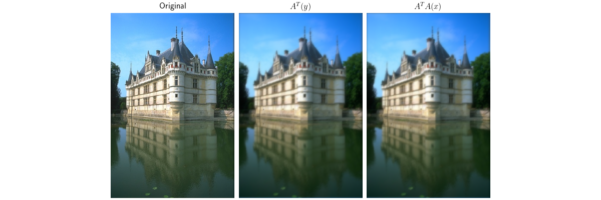
        # Plot adjoint and A^T A results
        # Normalize for visualization
        adjoint_vis = (adjoint_result - adjoint_result.min()) / (
            adjoint_result.max() - adjoint_result.min() + 1e-8
        )
        ata_vis = (ata_result - ata_result.min()) / (
            ata_result.max() - ata_result.min() + 1e-8
        )

        plot(
            [clean_image, adjoint_vis, ata_vis],
            titles=["Original", r"$A^T(y)$", r"$A^T A(x)$"],
            save_fn="distributed_physics_adjoint.png",
            figsize=(12, 4),
        )

        print(f"\n Demo completed successfully!")
        print(f"   Results saved to:")
        print(f"   - distributed_physics_forward.png")
        print(f"   - distributed_physics_adjoint.png")
        print("\n" + "=" * 70)

• 
• 

======================================================================
Distributed Physics Operators Demo
======================================================================

Running on 1 process(es)
   Device: cuda:0

Created stacked physics with 3 operators
   Image shape: torch.Size([1, 3, 767, 512])
   Operator types: ['Blur', 'Blur', 'Blur']

 Distributed physics created
   Local operators on this rank: 3

 Testing forward operation (A)...
   Output type: TensorList
   Number of measurements: 3
   Measurement 0 shape: torch.Size([1, 3, 767, 512])
   Measurement 1 shape: torch.Size([1, 3, 767, 512])
   Measurement 2 shape: torch.Size([1, 3, 767, 512])

 Comparing with non-distributed forward operation...
   Mean absolute difference: 0.00e+00
   Max absolute difference:  0.00e+00
   Results match exactly!

Testing adjoint operation (A^T)...
   Output shape: torch.Size([1, 3, 767, 512])
   Output norm: 1663.4261

Comparing with non-distributed adjoint operation...
   Mean absolute difference: 0.00e+00
   Max absolute difference:  0.00e+00
   Results match exactly!

Testing composition (A^T A)...
   Output shape: torch.Size([1, 3, 767, 512])
   Output norm: 1663.4261

Comparing with non-distributed A^T A operation...
   Mean absolute difference: 0.00e+00
   Max absolute difference:  0.00e+00
   Results match exactly!

Visualizing results...

 Demo completed successfully!
   Results saved to:
   - distributed_physics_forward.png
   - distributed_physics_adjoint.png

======================================================================