Inverse scattering problem

In this example we show how to use the deepinv.physics.Scattering forward model.

The scattering inverse problem consists in reconstructing the contrast of an unknown object from measurements of the scattered wave field resulting from the interaction of an incident wave with the object.

For each of the \(i=1,\dots,T\) transmitters, the 2D forward model is given by inhomogeneous Helmholtz equation (see e.g., Soubies et al. [97]):

\[\nabla^2 u_i(\mathbf{r}) + k^2(\mathbf{r}) u_i(\mathbf{r}) = - (k^2(\mathbf{r}) - k^2_b) v_i(\mathbf{r}) \quad \mathbf{r} \in \mathbb{R}^2\]

where \(u_i\) is the (unknown) scattered field, \(k_b\) is the (known scalar) wavenumber of the incident wave in the background medium, \(k(\mathbf{r})\) is the (unknown) spatially-varying wavenumber of the object to be recovered, and \(v_i\) is the incident field generated by the ith transmitter in the absence of the object. The total field (scattered + incident) is measured at \(R\) different receiver locations surrounding the object.

Parametrizing the unknown spatially-varying wavenumber as \(k^2(\mathbf{r}) = k_b^2 (x(\mathbf{r})+1)\), where \(k_b\) is the background wavenumber, and \(x = k^2/k_b^2 - 1\) is the scattering potential of the object to be recovered, the forward problem can be reformulated in the Lippmann-Schwinger integral equation form:

\[\begin{split}u_i &= g * \left( x \circ (u_i+v_i) \right) \\ y_i &= G_s \left( x \circ (u_i+v_i) \right)\end{split}\]

where \(g(\mathbf{r}) = k_b^2 \frac{i}{4} H_0^1(k_b\|\mathbf{r}\|)\) is Green’s function in 2D (normalized by \(k_b^2\)), \(y \in \mathbb{C}^{R}\) are the measurements at the receivers for the ith transmitter, and \(G_s\) denotes the convolution with Green’s operator plus sampling at the \(R\) different receiver locations.

Tip

This parametrization ensures that the scattering potential \(x\) is dimensionless, and can be used for different physical modalities: In microwave tomography applications, the scattering potential is related to the object’s relative permittivity \(\epsilon_r\) as \(x(\mathbf{r}) = \epsilon_r(\mathbf{r}) - 1\). In optical diffraction tomography, the scattering potential is related to the refractive index \(n\) as \(x(\mathbf{r}) = n^2(\mathbf{r}) - 1\).

Moreover, the wavenumber can be also provided in a dimensionless form by normalizing it with respect to the box length \(L\) as \(k_b = 2 \pi L / \lambda\), where \(\lambda\) is the wavelength of the incident wave.

This example shows how to define the scattering forward model, generate measurements, and perform reconstructions (i.e., recover the contrast of the object) using both a linear (Born approximation) solver and a non-linear gradient descent solver. We also explore the trade-off between resolution and non-linearity by varying the wavenumber of the incident wave.

import deepinv as dinv
import torch
from matplotlib import pyplot as plt

device = dinv.utils.get_freer_gpu() if torch.cuda.is_available() else "cpu"

img_width = 32

x = dinv.utils.load_example(
    "SheppLogan.png",
    img_size=img_width,
    resize_mode="resize",
    device=device,
    grayscale=True,
)

contrast = (
    0.5 if device != "cpu" else 0.1
)  # reduce contrast for CPU for faster convergence
x = x * contrast

psnr = dinv.metric.PSNR(max_pixel=contrast)

Selected GPU 0 with 8055.25 MiB free memory

Define the forward model

We define a scattering forward model with circularly distributed transmitters and receivers.

The forward operator internally solves the Lippmann-Schwinger equation for the scattered field of each transmitter:

\[u_i = g * \left(x \circ (u_i + v_i) \right)\]

using a linear system solver, which aims at finding the solution \(u_i\) of

\[\left(I - G_s \text{diag}(x)\right) u_i = b_i\]

where \(G_s\) is the convolution operator with Green’s function \(g\), and \(b_i = G_s (x \circ v_i)\).

This linear system becomes highly ill-conditioned for high contrast objects (i.e., large \(\|x\|_{\infty}\)) and/or high wavenumber (which induces a high spectral norm of the Green operator \(\|G_s\|_2\)), and the solver may fail to converge. In that case, one can try to increase the number of iterations, or change the solver (see deepinv.physics.Scattering.SolverConfig for more details).

sensors = 32
transmitters, receivers = dinv.physics.scattering.circular_sensors(
    sensors, radius=1, device=device
)
wavenumber = 5 * (2 * torch.pi)

config = dinv.physics.Scattering.SolverConfig(
    max_iter=200, tol=1e-5, solver="lsqr", adjoint_state=True
)

physics = dinv.physics.Scattering(
    img_width=img_width,
    device=device,
    background_wavenumber=wavenumber,
    solver_config=config,
    transmitters=transmitters,
    receivers=receivers,
)
physics.normalize(x)


physics.set_verbose(True)
y = physics(x)

LSQR converged at iteration 24

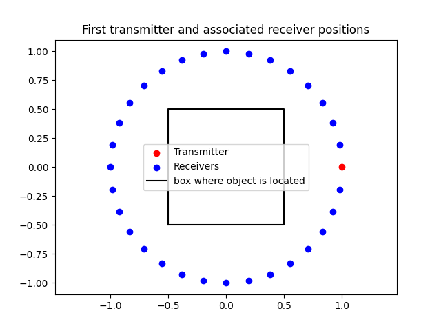
Visualize sensor positions

In this example, we assume we have 64 sensors that can be used both as transmitters and receivers, placed on a circle of radius 1 around the object. Each transmitter emits a cylindrical wave, and the rest of the sensors measure the scattered field. We first visualize the position of the first transmitter and its associated receivers.

plt.figure()
plt.scatter(
    transmitters[0, 0].cpu(), transmitters[1, 0].cpu(), c="r", label="Transmitter"
)
plt.scatter(
    receivers[0, 0, :].cpu(), receivers[1, 0, :].cpu(), c="b", label="Receivers"
)
# draw square of length1
plt.plot(
    [-0.5, 0.5, 0.5, -0.5, -0.5],
    [-0.5, -0.5, 0.5, 0.5, -0.5],
    c="k",
    label="box where object is located",
)
plt.legend()
plt.title("First transmitter and associated receiver positions")
plt.axis("equal")
plt.show()

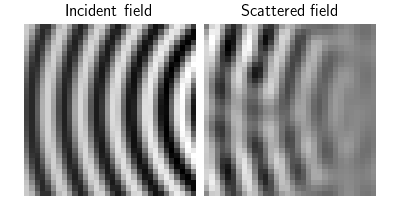
Visualize incident and total fields

We now visualize the incident and scattered fields for the first transmitter. The incident field \(v_i\) is the field that would be present in the absence of the object, while the total field \(u_i + v_i\) is the sum of the incident and scattered fields.

Since the fields are complex-valued, we only visualize their real part here.

incident_field = physics.incident_field
scattered_field = physics.compute_total_field(x) - incident_field
dinv.utils.plot(
    [incident_field[:, :1, ...].real, scattered_field[:, :1, ...].real],
    titles=["Incident field", "Scattered field"],
    figsize=(4, 2),
)

LSQR converged at iteration 24

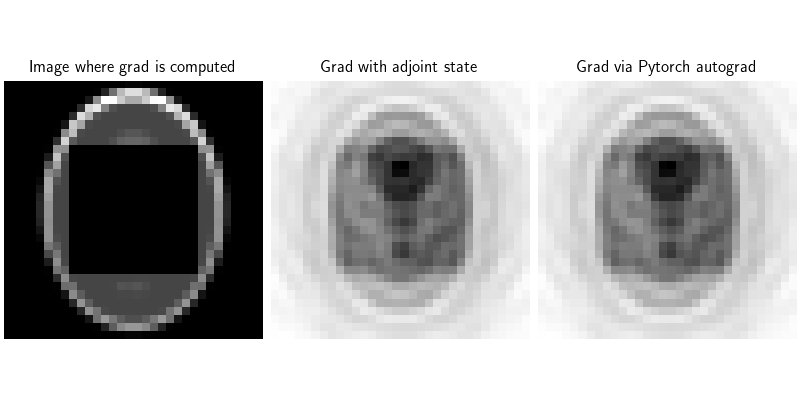
Computing gradients through the physics operator

The gradient computation is fully compatible with PyTorch autograd, allowing to easily plug this physics operator into more complex optimization or learning-based algorithms.

Gradients can be computed with less memory using the adjoint-state method under the hood, requiring a single additional solver pass per gradient evaluation (see e.g. Soubies et al. [97]), and does not require storing all intermediate variables (as in standard backpropagation via PyTorch autograd). Here we show that the gradients computed using the adjoint-state method are consistent with those computed via standard PyTorch autograd.

Note

If you are using a GPU, the peak memory usage during gradient computation is also displayed for comparison.

def compute_grad(x, y, physics):
    if device != "cpu":
        torch.cuda.reset_peak_memory_stats()  # Reset peak memory tracking

    x_ = x.clone()
    x_[
        ..., img_width // 4 : 3 * img_width // 4, img_width // 4 : 3 * img_width // 4
    ] = 0.0
    x_ = x_.requires_grad_(True)
    y_ = physics.A(x_)
    error = torch.mean((y_ - y).abs() ** 2)
    grad = torch.autograd.grad(error, x_)[0]

    if device != "cpu":
        print(
            f"Peak GPU memory usage for grad computation: "
            f"{torch.cuda.max_memory_allocated() / 1e6 :.1f} MB",
        )
    return x_, grad


x_, grad = compute_grad(x, y, physics)
# set solver to not use adjoint state
config2 = dinv.physics.Scattering.SolverConfig(
    max_iter=200, tol=1e-5, solver="lsqr", adjoint_state=False
)
physics.set_solver(config2)
_, grad2 = compute_grad(x, y, physics)

dinv.utils.plot(
    [x_.real, grad, grad2],
    titles=[
        "Image where grad is computed",
        "Grad with adjoint state",
        "Grad via Pytorch autograd",
    ],
    figsize=(8, 4),
)

print("Difference between gradients:", (grad - grad2).abs().mean().item())

# go back to adjoint state solver
physics.set_solver(config)

LSQR converged at iteration 22
LSQR converged at iteration 22
Peak GPU memory usage for grad computation: 61.3 MB
Peak GPU memory usage for grad computation: 180.2 MB
Difference between gradients: 1.0060698940606017e-09

Reconstruction with linear (Born approximation) solver

The born (first-order) approximation consists in assuming that the scattered field is small compared to the incident field, i.e., \(u_i \ll v_i\). This allows to approximate the Lippmann-Schwinger equation as:

\[y_i = G_s \left(x \circ v_i\right)\]

which is a linear forward model in \(x\). This linear model can be inverted using its linear pseudo-inverse, computed with a linear solver.

physics.set_verbose(False)

x_lin = physics.A_dagger(y, linear=True)

print(f"PSNR of Born approximation: {psnr(x, x_lin).item():2f} dB")

PSNR of Born approximation: 14.431273 dB

Reconstruction with gradient descent

The linear Born approximation is only valid for weakly scattering objects. We now perform a non-linear reconstruction using gradient descent to minimize the least-squares data-fidelity term:

\[\min_x \frac{1}{2} \sum_{i=1}^T \| y_i - A_i(x) \|_2^2\]

where \(A_i(x)\) is the non-linear forward operator for the ith transmitter, given by the Lippmann-Schwinger equation above.

Note

We can use a step size of 1 here since we have normalized the physics operator to have a (local) Lipschitz constant of 1.

Note

Here we only do 50 iterations for demonstration purposes. In practice, more iterations may be needed to reach convergence.

data_fid = dinv.optim.L2()
gd_solver = dinv.optim.GD(
    max_iter=50,
    data_fidelity=data_fid,
    stepsize=1,
    custom_init=lambda y, physics: physics.A_dagger(y, linear=True),
)

x_gd = gd_solver(y, physics)

print(f"PSNR of gradient descent reconstruction: {psnr(x, x_gd).item():.2f} dB")

dinv.utils.plot(
    [x, x_lin, x_gd],
    titles=[
        "ground truth",
        f"Born approximation\nPSNR={psnr(x, x_lin).item():.2f}dB",
        f"Gradient descent\nPSNR={psnr(x, x_gd).item():.2f}dB",
    ],
    figsize=(10, 3),
)

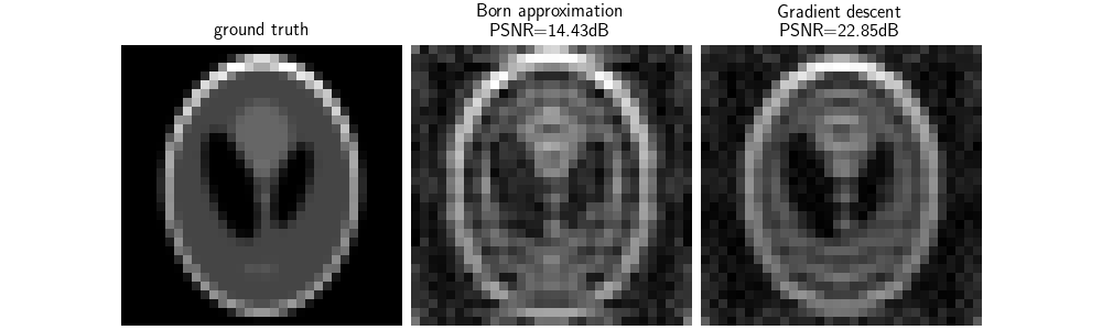
PSNR of gradient descent reconstruction: 22.85 dB

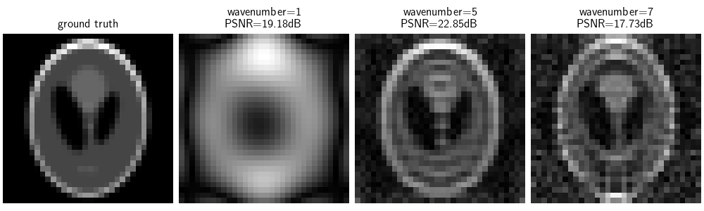
Understanding the trade-off between resolution and non-linearity

The background wavenumber \(k_b\) (or equivalently the frequency) of the transmitted wave plays a key role in the scattering process. Higher wavenumbers lead to smaller waves which can resolve smaller details in the object being imaged. However, higher wavenumbers also lead to stronger multiple scattering effects, since the non-linearity of the problem is roughly proportional to \(\|x\|_{\infty} k_b\) (i.e., the product of the object contrast and the wavenumber).

We now compare the Born approximation reconstruction with a gradient descent reconstruction for different normalized wavenumbers (i.e. different resolutions).

Note

This example requires a GPU to run in a reasonable time.

if device != "cpu":

    imgs = [x.detach().cpu()]
    titles = ["ground truth"]

    wavenumbers = [1, 5, 7]
    for wavenumber in wavenumbers:
        physics = dinv.physics.Scattering(
            img_width=img_width,
            device=device,
            background_wavenumber=wavenumber * (2 * torch.pi),
            transmitters=transmitters,
            receivers=receivers,
        )
        physics.normalize(x)
        y = physics(x)

        x_gd = gd_solver(y, physics)

        metric = psnr(x_gd, x)
        titles = titles + [f"wavenumber={wavenumber} \n PSNR={metric.item():.2f}dB"]
        imgs = imgs + [x_gd.detach().cpu()]

    dinv.utils.plot(imgs, titles=titles, figsize=(10, 3))

Going further

You can check out the following examples to go further:

• Try other sensor configurations, e.g., a linear array of transmitters on one side of the object, and receivers on the opposite side.

• Use a pretrained denoiser to perform plug-and-play reconstruction, as in Vanilla PnP for computed tomography (CT).

• Learn a reconstruction network using an unrolled architecture, as in Vanilla Unfolded algorithm for super-resolution.

References: