Blind denoising with noise level estimation

This example focuses on blind image Gaussian denoising, i.e. the problem

\[y = x + \sigma n \quad n \sim \mathcal{N}(0, I)\]

where \(\sigma\) is unknown. In this example, we first propose to estimate the noise level with different approaches, and then show general restoration models available in the library.

import torch
import deepinv as dinv

device = dinv.utils.get_freer_gpu() if torch.cuda.is_available() else "cpu"

Selected GPU 0 with 4096.25 MiB free memory

Build a noisy image

We load a noiseless image and generate a noisy (Gaussian) version of this image, with standard deviation that we will assume to be unknown. We set it to \(\sigma = 0.042\) for this example.

x = dinv.utils.load_example("butterfly.png", device=device)

sigma_true = 0.042

y = x + sigma_true * torch.randn_like(x)

A naive approach

A first naive approach to estimate \(\sigma\) consists in taking a patch of the image, removing the mean, and using the standard deviation of the resulting patch as an estimate of the noise level.

p = 50
y_patch = y[:, :, -p:, p - p // 2 : p + p // 2]  # extract a patch
std_naive = y_patch.std()

print("Naive noise level estimate: ", std_naive.item())

Naive noise level estimate:  0.15947508811950684

Noise level estimators

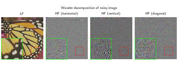
A more advanced approach consists in performing the same approach as above, but in an appropriate domain. A good transform is the wavelet transform, where we can expect the noise to dominate high-frequency components. We can illustrate this as follows:

import ptwt
import pywt

coeffs = ptwt.wavedec2(y, pywt.Wavelet("db8"), mode="constant", level=1, axes=(-2, -1))

imgs = [coeffs[0], coeffs[1][0], coeffs[1][1], coeffs[1][2]]
titles = ["LF", "HF (horizontal)", "HF (vertical)", "HF (diagonal)"]

dinv.utils.plot_inset(
    img_list=imgs,
    titles=titles,
    suptitle="Wavelet decomposition of noisy image",
    extract_size=0.2,
    extract_loc=(0.7, 0.7),
    inset_size=0.5,
    figsize=(len(imgs) * 1.5, 2.5),
    fontsize=8,
)

/local/jtachell/deepinv/deepinv/deepinv/utils/plotting.py:408: UserWarning: This figure was using a layout engine that is incompatible with subplots_adjust and/or tight_layout; not calling subplots_adjust.
  fig.subplots_adjust(top=0.75)

We notice that the high-frequency components are mostly noise. We can thus use these components to estimate the noise level more robustly. This is implemented in deepinv.models.WaveletNoiseEstimator. Under the hood, the estimator uses the Median Absolute Deviation (MAD) estimator on the wavelet high-frequency coefficients:

\[\qquad \hat{\sigma} = \frac{\mathrm{median}(|w|)}{0.6745},\]

where \(w\) are the high-frequency wavelet coefficients.

wavelet_estimator = dinv.models.WaveletNoiseEstimator()
sigma_wavelet = wavelet_estimator(y)
print("Wavelet-based noise level estimate: ", sigma_wavelet.item())

Wavelet-based noise level estimate:  0.05336251109838486

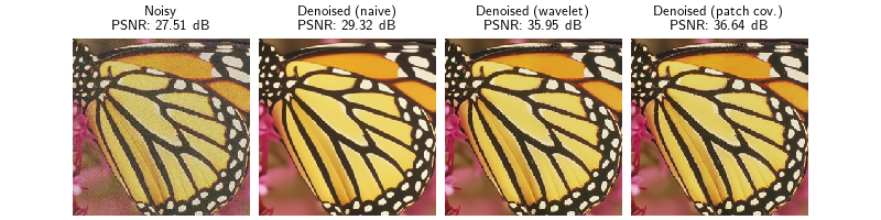
We notice that this approach provides a signficantly better estimate of the noise level compared to the naive approach. However, it tends to slightly over-estimate the noise level in this example. As noted in the original paper, this is due to the presence of residual signal in the high-frequency wavelet coefficients (these are not only noise).

Another approach is to use the eigenvalues of the covariance matrix of patches extracted from the noisy image. This is implemented in deepinv.models.PatchCovarianceNoiseEstimator. The method was initially proposed in Chen et al.[1].

patch_cov_estimator = dinv.models.PatchCovarianceNoiseEstimator()
sigma_patch_cov = patch_cov_estimator(y)
print("Patch covariance-based noise level estimate: ", sigma_patch_cov.item())

Patch covariance-based noise level estimate:  0.04178362712264061

Blind denoising with estimated noise level

Once we have estimated the noise level, we can use general denoising models available in the library. Here, we use the pretrained DRUNet model from Zhang et al.[2] that can handle a range of noise levels.

denoiser = dinv.models.DRUNet(device=device)

with torch.no_grad():
    denoised_naive = denoiser(y, sigma=std_naive)
    denoised_wavelet = denoiser(y, sigma=sigma_wavelet)
    denoised_patch_cov = denoiser(y, sigma=sigma_patch_cov)


metric = dinv.metric.PSNR()

psnr_noisy = metric(y, x).item()
psnr_naive = metric(denoised_naive, x).item()
psnr_wavelet = metric(denoised_wavelet, x).item()
psnr_patch_cov = metric(denoised_patch_cov, x).item()

dinv.utils.plot(
    {
        f"Noisy\n PSNR: {psnr_noisy:.2f} dB": y,
        f"Denoised (naive)\n PSNR: {psnr_naive:.2f} dB": denoised_naive,
        f"Denoised (wavelet)\n PSNR: {psnr_wavelet:.2f} dB": denoised_wavelet,
        f"Denoised (patch cov.)\n PSNR: {psnr_patch_cov:.2f} dB": denoised_patch_cov,
    },
    fontsize=9,
)

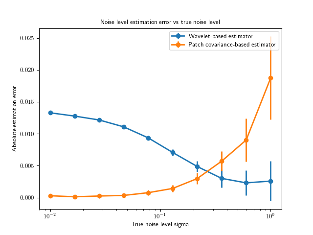
Which noise level estimator is best?

This will depend on several parameters, e.g. image size, content and noise level. Above, the patch covariance estimator provides the best results. We can investigate the performance on the above image for different noise levels as follows:

list_sigmas = torch.logspace(-2, 0, steps=10)

estimate_errors = {
    "wavelet mean": [],
    "wavelet std": [],
    "patch_cov mean": [],
    "patch_cov std": [],
}

mean_abs_error = dinv.metric.MAE(reduction="mean")

# run estimations for different noise levels, and average over 10 random seeds
for sigma in list_sigmas:

    sigma_wavelet, sigma_patch_cov = [], []

    for seed in range(10):
        torch.manual_seed(seed)
        y_ = x + sigma * torch.randn_like(x)

        sigma_wavelet.append(wavelet_estimator(y_))
        sigma_patch_cov.append(patch_cov_estimator(y_))

    sigma_wavelet = torch.stack(sigma_wavelet)
    sigma_patch_cov = torch.stack(sigma_patch_cov)

    estimate_errors["wavelet mean"].append(mean_abs_error(sigma_wavelet, sigma).item())
    estimate_errors["wavelet std"].append(sigma_wavelet.std().item())
    estimate_errors["patch_cov mean"].append(
        (sigma_patch_cov - sigma).abs().mean().item()
    )
    estimate_errors["patch_cov std"].append(sigma_patch_cov.std().item())

# plot results
import matplotlib.pyplot as plt

plt.figure()
plt.errorbar(
    list_sigmas.cpu(),
    estimate_errors["wavelet mean"],
    yerr=estimate_errors["wavelet std"],
    label="Wavelet-based estimator",
    fmt="-o",
)
plt.errorbar(
    list_sigmas.cpu(),
    estimate_errors["patch_cov mean"],
    yerr=estimate_errors["patch_cov std"],
    label="Patch covariance-based estimator",
    fmt="-o",
)
plt.xscale("log")
plt.xlabel("True noise level sigma")
plt.ylabel("Absolute estimation error")
plt.title("Noise level estimation error vs true noise level")
plt.legend()
plt.show()

Blind denoising models

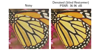
Finally, we can also use blind denoising models that are trained to denoise images without knowing the noise level. For instance, we can use the Restormer model from Zamir et al.[3]. We note that this model provides better results than the non-blind denoiser with estimated noise level.

blind_restormer = dinv.models.Restormer(device=device)

with torch.no_grad():
    denoised_restormer = blind_restormer(y)

psnr_restormer = metric(denoised_restormer, x).item()

dinv.utils.plot(
    {
        "Noisy": y,
        f"Denoised (blind Restormer)\n PSNR: {psnr_restormer:.2f} dB": denoised_restormer,
    },
    fontsize=9,
)

Loading from gaussian_color_denoising_blind.pth

References:

[1]

Guangyong Chen, Fengyuan Zhu, and Pheng Ann Heng. An efficient statistical method for image noise level estimation. In Proceedings of the IEEE international conference on computer vision, 477–485. 2015.

[2]

Kai Zhang, Yawei Li, Wangmeng Zuo, Lei Zhang, Luc Van Gool, and Radu Timofte. Plug-and-play image restoration with deep denoiser prior. IEEE Transactions on Pattern Analysis and Machine Intelligence, 44(10):6360–6376, 2021.

[3]

Syed Waqas Zamir, Aditya Arora, Salman Khan, Munawar Hayat, Fahad Shahbaz Khan, and Ming-Hsuan Yang. Restormer: efficient transformer for high-resolution image restoration. In Proceedings of the IEEE/CVF conference on computer vision and pattern recognition, 5728–5739. 2022.