Flow-Matching for posterior sampling and unconditional generation#

This demo shows you how to perform unconditional image generation and posterior sampling using Flow Matching (FM).

Flow matching consists in building a continuous transportation between a reference distribution \(p_1\) which is easy to sample from (e.g., a Gaussian distribution) and the data distribution \(p_0\). Sampling is done by solving the following ordinary differential equation (ODE) defined by a time-dependent velocity field \(v_\theta(x,t)\):

\[\frac{dx_t}{dt} = v_\theta(x_t,t), \quad x_0 \sim p_0 \quad t \in [0,1]\]

The velocity field \(v_\theta(x,t)\) is typically trained to approximate the conditional expectation:

\[v_\theta(x_t,t) \approx \mathbb{E}_{x_0 \sim p_0, x_1 \sim p_1}\Big[ \frac{d}{dt} x_t | x_t = a(t) x_0 + b(t) x_1 \Big]\]

where \(a(t)\) and \(b(t)\) are interpolation coefficients such that \(x_t\) interpolates between \(x_0\) and \(x_1\). When the reference distribution \(p_0\) is the standard Gaussian, the velocity field can be expressed as a function of a Gaussian denoiser \(D(x, \sigma)\) as follows:

\[v_\theta(x_t,t) = - \frac{b'(t)}{b(t)} x_t + \frac{1}{2}\frac{a(t) b'(t) - a'(t) b(t)}{a(t) b(t)} \left(D\left(\frac{x_t}{a(t)}, \frac{b(t)}{a(t)} \right) - x_t\right)\]

The most common choice of time schedulers is the linear schedule \(a(t) = 1 - t\) and \(b(t) = t\).

In this demo, we will show how to :

Perform unconditional generation using, instead of a trained denoiser, the closed-form MMSE denoiser

\[D(x, \sigma) = \mathbb{E}_{x_0 \sim p_{data}, \epsilon \sim \mathcal{N}(0, I)} \Big[ x_0 | x = x_0 + \sigma \epsilon \Big]\]

Given a dataset of clean images, it can be computed by evaluating the distance between the input image and all the points of the dataset (see deepinv.models.MMSE).

Perform posterior sampling using Flow-Matching combined with a DPS data fidelity term (see Building your diffusion posterior sampling method using SDEs for more details)
Explore different choices of time schedulers \(a(t)\) and \(b(t)\).

import torch
import deepinv as dinv
from deepinv.sampling import (
    PosteriorDiffusion,
    DPSDataFidelity,
    EulerSolver,
    FlowMatching,
)
import numpy as np
from torchvision import datasets, transforms
from deepinv.models import MMSE

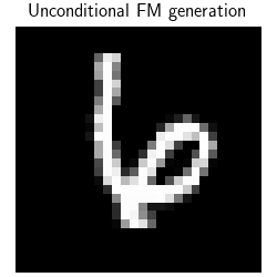
We start by working with the closed-form MMSE denoser. It is calculated by computing the distance between the input image and all the points of the dataset. This can be quite long to compute for large images and large datasets. In this toy example, we use the validation set of MNIST. When using this closed-form MMSE denoiser, the sampling is guaranteed to output an image of the dataset.

device = dinv.utils.get_device()
dtype = torch.float32

figsize = 2.5

# We use the closed-form MMSE denoiser defined using as atoms the testset of MNIST.
# The deepinv MMSE denoiser takes as input a dataloader.
dataset = datasets.MNIST(
    root=".", train=False, download=True, transform=transforms.ToTensor()
)
dataloader = torch.utils.data.DataLoader(dataset, batch_size=1000, shuffle=False)
n_max = (
    1000  # limit the number of images to speed up the computation of the MMSE denoiser
)
tensors = torch.cat([data[0] for data in iter(dataloader)], dim=0)  # (N,1,28,28)
tensors = tensors[:n_max].to(device)
denoiser = MMSE(dataloader=tensors, device=device, dtype=dtype)

Selected GPU 0 with 4989.25 MiB free memory

  0%|          | 0.00/9.91M [00:00<?, ?B/s]
  1%|          | 98.3k/9.91M [00:00<00:19, 501kB/s]
  3%|▎         | 262k/9.91M [00:00<00:13, 697kB/s]
  5%|▍         | 459k/9.91M [00:00<00:11, 836kB/s]
  7%|▋         | 688k/9.91M [00:00<00:09, 966kB/s]
  9%|▉         | 918k/9.91M [00:00<00:08, 1.04MB/s]
 11%|█         | 1.08M/9.91M [00:01<00:07, 1.16MB/s]
 13%|█▎        | 1.28M/9.91M [00:01<00:07, 1.11MB/s]
 15%|█▍        | 1.47M/9.91M [00:01<00:06, 1.29MB/s]
 17%|█▋        | 1.64M/9.91M [00:01<00:06, 1.26MB/s]
 18%|█▊        | 1.80M/9.91M [00:01<00:06, 1.19MB/s]
 20%|█▉        | 1.93M/9.91M [00:01<00:06, 1.22MB/s]
 22%|██▏       | 2.20M/9.91M [00:01<00:06, 1.27MB/s]
 24%|██▍       | 2.36M/9.91M [00:02<00:05, 1.35MB/s]
 26%|██▌       | 2.59M/9.91M [00:02<00:04, 1.57MB/s]
 28%|██▊       | 2.79M/9.91M [00:02<00:05, 1.35MB/s]
 30%|███       | 3.01M/9.91M [00:02<00:04, 1.44MB/s]
 32%|███▏      | 3.18M/9.91M [00:02<00:05, 1.32MB/s]
 34%|███▎      | 3.34M/9.91M [00:02<00:04, 1.39MB/s]
 36%|███▌      | 3.57M/9.91M [00:02<00:04, 1.48MB/s]
 38%|███▊      | 3.77M/9.91M [00:03<00:04, 1.40MB/s]
 40%|███▉      | 3.96M/9.91M [00:03<00:03, 1.53MB/s]
 42%|████▏     | 4.16M/9.91M [00:03<00:03, 1.50MB/s]
 44%|████▎     | 4.33M/9.91M [00:03<00:04, 1.35MB/s]
 46%|████▌     | 4.52M/9.91M [00:03<00:03, 1.49MB/s]
 48%|████▊     | 4.72M/9.91M [00:03<00:03, 1.61MB/s]
 50%|████▉     | 4.92M/9.91M [00:03<00:03, 1.37MB/s]
 52%|█████▏    | 5.11M/9.91M [00:03<00:03, 1.50MB/s]
 54%|█████▍    | 5.34M/9.91M [00:04<00:02, 1.56MB/s]
 56%|█████▌    | 5.54M/9.91M [00:04<00:03, 1.45MB/s]
 58%|█████▊    | 5.77M/9.91M [00:04<00:02, 1.52MB/s]
 60%|█████▉    | 5.93M/9.91M [00:04<00:02, 1.37MB/s]
 61%|██████▏   | 6.09M/9.91M [00:04<00:02, 1.43MB/s]
 63%|██████▎   | 6.29M/9.91M [00:04<00:02, 1.56MB/s]
 65%|██████▌   | 6.49M/9.91M [00:04<00:02, 1.53MB/s]
 67%|██████▋   | 6.65M/9.91M [00:05<00:02, 1.36MB/s]
 69%|██████▉   | 6.82M/9.91M [00:05<00:02, 1.43MB/s]
 71%|███████   | 7.01M/9.91M [00:05<00:01, 1.56MB/s]
 73%|███████▎  | 7.21M/9.91M [00:05<00:01, 1.53MB/s]
 75%|███████▍  | 7.41M/9.91M [00:05<00:01, 1.43MB/s]
 77%|███████▋  | 7.60M/9.91M [00:05<00:01, 1.56MB/s]
 79%|███████▊  | 7.80M/9.91M [00:05<00:01, 1.52MB/s]
 80%|████████  | 7.96M/9.91M [00:05<00:01, 1.37MB/s]
 82%|████████▏ | 8.13M/9.91M [00:05<00:01, 1.43MB/s]
 84%|████████▎ | 8.29M/9.91M [00:06<00:01, 1.48MB/s]
 86%|████████▌ | 8.49M/9.91M [00:06<00:00, 1.61MB/s]
 88%|████████▊ | 8.68M/9.91M [00:06<00:00, 1.56MB/s]
 89%|████████▉ | 8.85M/9.91M [00:06<00:00, 1.38MB/s]
 91%|█████████ | 9.04M/9.91M [00:06<00:00, 1.52MB/s]
 93%|█████████▎| 9.21M/9.91M [00:06<00:00, 1.55MB/s]
 95%|█████████▌| 9.44M/9.91M [00:06<00:00, 1.60MB/s]
 97%|█████████▋| 9.63M/9.91M [00:06<00:00, 1.47MB/s]
 99%|█████████▉| 9.83M/9.91M [00:07<00:00, 1.59MB/s]
100%|██████████| 9.91M/9.91M [00:07<00:00, 1.39MB/s]

  0%|          | 0.00/28.9k [00:00<?, ?B/s]
100%|██████████| 28.9k/28.9k [00:00<00:00, 303kB/s]

  0%|          | 0.00/1.65M [00:00<?, ?B/s]
  6%|▌         | 98.3k/1.65M [00:00<00:03, 513kB/s]
 18%|█▊        | 295k/1.65M [00:00<00:01, 815kB/s]
 32%|███▏      | 524k/1.65M [00:00<00:01, 988kB/s]
 46%|████▌     | 754k/1.65M [00:00<00:00, 1.07MB/s]
 62%|██████▏   | 1.02M/1.65M [00:00<00:00, 1.18MB/s]
 78%|███████▊  | 1.28M/1.65M [00:01<00:00, 1.24MB/s]
 93%|█████████▎| 1.54M/1.65M [00:01<00:00, 1.28MB/s]
100%|██████████| 1.65M/1.65M [00:01<00:00, 1.23MB/s]

  0%|          | 0.00/4.54k [00:00<?, ?B/s]
100%|██████████| 4.54k/4.54k [00:00<00:00, 11.4MB/s]

The FlowMatching module deepinv.sampling.FlowMatching uses by default the following schedules: \(a_t=1-t\), \(b_t=t\). The module FlowMatching module takes as input the denoiser and the ODE solver.

num_steps = 100
timesteps = torch.linspace(0.99, 0.0, num_steps)
rng = torch.Generator(device).manual_seed(5)
solver = EulerSolver(timesteps=timesteps, rng=rng)
sde = FlowMatching(denoiser=denoiser, solver=solver, device=device, dtype=dtype)


sample, trajectory = sde(
    x_init=(1, 1, 28, 28),
    seed=0,
    get_trajectory=True,
)

dinv.utils.plot(
    sample,
    titles="Unconditional FM generation",
    save_fn="FM_sample.png",
    figsize=(figsize, figsize),
)

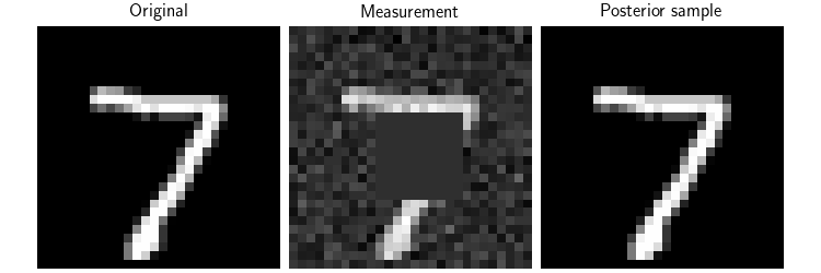
Now, we can use the Flow-Matching model to perform posterior sampling. We consider the inpainting problem, where we have a masked image and we want to recover the original image. We use DPS deepinv.sampling.DPSDataFidelity as data fidelity term (see Building your diffusion posterior sampling method using SDEs for more details). Note that due to the division by \(a(t)\) in the velocity field, initialization close to t=1 causes instability.

x = next(iter(dataloader))[0][:1].to(device)

mask = torch.ones_like(x)
mask[..., 10:20, 10:20] = 0.0
physics = dinv.physics.Inpainting(
    img_size=x.shape[1:],
    mask=mask,
    device=device,
    noise_model=dinv.physics.GaussianNoise(sigma=0.1),
)
y = physics(x)
dps_fidelity = DPSDataFidelity(denoiser=denoiser, weight=1.0)
model = PosteriorDiffusion(
    data_fidelity=dps_fidelity,
    sde=sde,
    solver=solver,
    dtype=dtype,
    device=device,
    verbose=True,
)
x_hat, trajectory = model(
    y,
    physics,
    x_init=None,
    get_trajectory=True,
    seed=0,
)

# Here, we plot the original image, the measurement and the posterior sample
dinv.utils.plot(
    [x, y, x_hat],
    show=True,
    titles=["Original", "Measurement", "Posterior sample"],
    figsize=(figsize * 3, figsize),
    save_fn="FM_posterior.png",
)

  0%|          | 0/99 [00:00<?, ?it/s]
 23%|██▎       | 23/99 [00:00<00:00, 221.17it/s]
 46%|████▋     | 46/99 [00:00<00:00, 200.57it/s]
 68%|██████▊   | 67/99 [00:00<00:00, 193.12it/s]
 88%|████████▊ | 87/99 [00:00<00:00, 188.50it/s]
100%|██████████| 99/99 [00:00<00:00, 192.01it/s]

Finally, we show how to use different choices of time schedulers \(a_t\) and \(b_t\). Here, we use another typical choice of schedulers \(a_t = \cos(\frac{\pi}{2} t)\) and \(b_t = \sin(\frac{\pi}{2} t)\) which also satisfy the interpolation condition \(a_0 = 1\), \(b_0 = 0\), \(a_1 = 0\), \(b_1 = 1\). Note that, again, due to the division by \(a_t\) in the velocity field, initialization close to t=1 causes instability.

a_t = lambda t: torch.cos(np.pi / 2 * t)
a_prime_t = lambda t: -np.pi / 2 * torch.sin(np.pi / 2 * t)
b_t = lambda t: torch.sin(np.pi / 2 * t)
b_prime_t = lambda t: np.pi / 2 * torch.cos(np.pi / 2 * t)

sde = FlowMatching(
    a_t=a_t,
    a_prime_t=a_prime_t,
    b_t=b_t,
    b_prime_t=b_prime_t,
    denoiser=denoiser,
    solver=solver,
    device=device,
    dtype=dtype,
)

model = PosteriorDiffusion(
    data_fidelity=dps_fidelity,
    sde=sde,
    solver=solver,
    dtype=dtype,
    device=device,
    verbose=True,
)

x_hat, trajectory = model(
    y,
    physics,
    x_init=None,
    get_trajectory=True,
)

# Here, we plot the original image, the measurement and the posterior sample
dinv.utils.plot(
    [x, y, x_hat],
    show=True,
    titles=["Original", "Measurement", "Posterior sample"],
    figsize=(figsize * 3, figsize),
    save_fn="FM_posterior_new_at_bt.png",
)

  0%|          | 0/99 [00:00<?, ?it/s]
 22%|██▏       | 22/99 [00:00<00:00, 212.36it/s]
 44%|████▍     | 44/99 [00:00<00:00, 191.64it/s]
 65%|██████▍   | 64/99 [00:00<00:00, 184.50it/s]
 84%|████████▍ | 83/99 [00:00<00:00, 181.82it/s]
100%|██████████| 99/99 [00:00<00:00, 184.13it/s]

References:

Total running time of the script: (0 minutes 18.662 seconds)

Gallery generated by Sphinx-Gallery

Flow-Matching for posterior sampling and unconditional generation#

This Page