Scattering

class deepinv.physics.Scattering(img_width, receivers, transmitters, background_wavenumber=10.0, solver_config=None, box_length=1.0, wave_type='circular_wave', device='cpu', dtype=torch.complex128, verbose=False)

Bases: Physics

Inverse scattering physics model in 2 dimensions.

For each of the \(i=1,\dots,T\) transmitters, the 2D forward model is given by inhomogeneous Helmholtz equation (see e.g., Soubies et al. [97]):

\[\nabla^2 u_i(\mathbf{r}) + k^2(\mathbf{r}) u_i(\mathbf{r}) = - (k^2(\mathbf{r}) - k^2_b) v_i(\mathbf{r}) \quad \mathbf{r} \in \mathbb{R}^2\]

where \(u_i\) is the (unknown) scattered field, \(k_b\) is the (known scalar) wavenumber of the incident wave in the background medium, \(k(\mathbf{r})\) is the (unknown) spatially-varying wavenumber of the object to be recovered, and \(v_i\) is the incident field generated by the ith transmitter in the absence of the object. The total field (scattered + incident) is measured at \(R\) different receiver locations surrounding the object.

Parametrizing the unknown spatially-varying wavenumber as \(k^2(\mathbf{r}) = k_b^2 (x(\mathbf{r})+1)\), where \(k_b\) is the background wavenumber, and \(x = k^2/k_b^2 - 1\) is the scattering potential of the object to be recovered, the problem can be reformulated in the Lippmann-Schwinger integral equation form:

\[\begin{split}u_i &= g * \left( x \circ (u_i+v_i) \right) \\ y_i &= G_s \left( x \circ (u_i+v_i) \right)\end{split}\]

where \(g(\mathbf{r}) = k_b^2 \frac{i}{4} H_0^1(k_b\|\mathbf{r}\|)\) is Green’s function in 2D (normalized by \(k_b^2\)), \(y \in \mathbb{C}^{R}\) are the measurements at the receivers for the ith transmitter, and \(G_s\) denotes the convolution with Green’s operator plus sampling at the \(R\) different receiver locations.

Tip

This parametrization ensures that the scattering potential \(x\) is dimensionless, and can be used for different physical modalities: In microwave tomography applications, the scattering potential is related to the object’s relative permittivity \(\epsilon_r\) as \(x(\mathbf{r}) = \epsilon_r(\mathbf{r}) - 1\). In optical diffraction tomography, the scattering potential is related to the refractive index \(n\) as \(x(\mathbf{r}) = n^2(\mathbf{r}) - 1\).

Moreover, the wavenumber can be also provided in a dimensionless form by normalizing it with respect to the box length \(L\) as \(k_b = 2 \pi L / \lambda\), where \(\lambda\) is the wavelength of the incident wave.

All spatial quantities are discretized in a square grid of size img_width x img_width pixels, which is assumed to cover a square domain of size \(L \times L\) in space, where \(L\) is the box length.

Note

The forward operator uses a linear solver to compute the total field for each transmitter by solving the Lippmann-Schwinger equation. The default solver configuration can be modified by passing a custom deepinv.physics.Scattering.SolverConfig object to the constructor. If the objects’ contrast and/or the wavenumber is very large, the linear solver may not converge, leading to inaccurate results. Setting verbose=True in the constructor will print solver convergence information, which can help diagnose convergence issues.

Note

The forward operator uses the adjoint state method to compute gradients, e.g., deepinv.physics.Scattering.A_jvp() and deepinv.physics.Scattering.A_vjp() by default, which is more memory efficient than using autograd, especially for large-scale problems. The adjoint state method requires one additional solve of the Lippmann-Schwinger equation per gradient computation, and avoids storing the entire computational graph (done by standard autograd). This can be disabled by setting adjoint_state=False in the deepinv.physics.Scattering.SolverConfig object passed to the constructor

Note

Green’s function has a singularity at r=0. In practice, we can avoid this issue following Vico et al. [112] which convolves Green’s function with a sinc kernel to account for the bounded domain:

\[g_L(\mathbf{r}) = g(\mathbf{r}) * \text{rect}\left(\frac{\|\mathbf{r}\|}{L}\right),\]

Parameters:

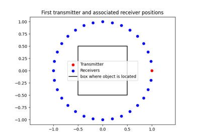
• img_width (int) – Number of pixels per image side (H=W). The minimum required number of pixels depends on the background wavenumber to avoid spatial aliasing. We require at least \(\text{image width} \geq 2 k_b L/(2 \pi)\), where \(k_b\) is the background wavenumber and \(L\) is the box length.

• receivers (torch.Tensor) – Tensor of shape (2, R) (shared receivers) or (2, T, R) (per-transmitter receivers) with receiver x/y positions (torch.float dtype).

• transmitters (torch.Tensor) – Tensor of shape (2, T) with transmitter x/y positions (torch.float dtype)

• background_wavenumber (float, torch.Tensor) – background wavenumber \(k_b\), which can be real (float or torch.float) or complex (torch.complex). It controls the frequency of the incident wave, and thus the maximum achievable resolution of the contrast image.

• solver_config (deepinv.physics.scattering.Scattering.SolverConfig) – Configuration for the Lippmann-Schwinger solver used to compute the total field (first equation in the forward model). If None, default configuration is used which uses the LSQR solver with a maximum of 500 iterations and tolerance 1e-5.

• box_length (float) – Physical side length of the square domain \(L\), which can be specified relative to the wavenumber.

• wave_type (str) – incident wave type. Options are 'circular_wave' or 'plane_wave'. The circular wave corresponds to a point source transmitter, while the plane wave corresponds to a far-field transmitter.

• device (str) – Torch device string, e.g. 'cpu' or 'cuda'.

• dtype (torch.dtype) – Torch dtype for tensors which must be of complex type (e.g. torch.complex128).

• verbose (bool) – Enable verbose/debug printing.

A(x, receivers=None, transmitters=None, **kwargs)

Forward operator wrapper: updates parameters, solves for total field and returns measurements.

Parameters:

• x (torch.Tensor) – Scattering potential (B,1,H,W).

• receivers (torch.Tensor) – Optional new receiver positions of shape (2, R) or (2, T, R).

• transmitters (torch.Tensor) – Optional new transmitter positions of shape (2, T), where T is the number of transmitters.

Returns:

(torch.Tensor) Measurements tensor of shape (B,T,R).

Return type:

Tensor

A_dagger(y, linear=False, x_init=None, max_iter=2, use_init=True, rel_tol=1e-3, **kwargs)

Pseudo-inverse for the scattering operator.

If linear=True, uses the Born approximation (single iteration).

If linear=False, alternates between updating the total field estimate with a fixed scattering potential, and updating the scattering potential estimate with a fixed total field, for a maximum of max_iter iterations.

Parameters:

• y (torch.Tensor) – Measurements tensor (B,T,R).

• linear (bool) – If True, use Born approximation (single iteration).

• x_init (torch.Tensor) – Initial guess for the reconstruction (B,1,H,W).

• max_iter (int) – Maximum number of alternating optimization iterations.

• use_init (bool) – If True, use previous total field estimate to initialize the next iteration.

• rel_tol (float) – Relative tolerance for convergence.

A_jvp(x, u, **kwargs)

Jacobian-vector product for the forward operator.

Parameters:

• x (torch.Tensor) – Scattering potential (B,1,H,W).

• u (torch.Tensor) – Vector to multiply with the Jacobian (B,1,H,W).

A_vjp(x, v, **kwargs)

Vector-Jacobian product for the forward operator.

Parameters:

• x (torch.Tensor) – Scattering potential of shape (B,1,H,W).

• v (torch.Tensor) – Vector to multiply with the Jacobian, a tensor of shape (B,T,R).

• dtype (torch.dtype) – torch.dtype used for internal computations and returned result

class SolverConfig(min_iter=1, max_iter=500, solver='lsqr', tol=1e-05, green_imaginary_part=0.0, adjoint_state=True, verbose=False)

Bases: object

Configuration class for the Lippmann-Schwinger solver.

Defines the parameters for the iterative solver used to solve the Lippmann-Schwinger equation.

Parameters:

• min_iter (int) – Minimum number of iterations. By default, 1.

• max_iter (int) – Maximum number of iterations. By default, 500.

• solver (str) – Linear solver to use ('lsqr', 'BiCGStab' or 'CG'). By default, 'lsqr'.

• tol (float) – Stopping criterion for the solver. By default, 1e-5.

• adjoint_state (bool) – If True, use adjoint state method for gradients, else use autograd. By default True.

• green_imaginary_part (float) – Small imaginary part to add to the wavenumber in the Green’s function to improve solver convergence. By default, 0 (no modification).

• verbose (bool) – If True, print solver convergence information. By default, False.

compute_field_out(x, total_field)

Compute sensor outputs \(y = G_s * ext{diag}(x) u\).

Parameters:

• x (torch.Tensor) – Scattering potential (B,1,H,W).

• total_field (torch.Tensor) – Total field u (B,T,H,W).

compute_total_field(x, **kwargs)

Solve for the total field given scattering potential x using the provided solver.

Parameters:

x (torch.Tensor) – Scattering potential tensor of shape (B,1,H,W).

Returns:

(torch.Tensor) Total field tensor of shape (B,T,H,W).

Return type:

Tensor

generate_incident_field(device, dtype)

Generate incident fields on the image grid and at receiver positions.

Plane waves are computed as:

\[v_i(\mathbf{r}) = \exp\left( \mathrm{i} \mathbf{k}_i^{\top} \mathbf{r} \right)\]

where \(\mathbf{k}_i\) is the wavevector for the ith transmitter.

Circular waves are computed using Green’s function as:

\[v_i(\mathbf{r}) = g(\|\mathbf{r} - \mathbf{r}_i\|)\]

where \(\mathbf{r}_i\) is the position of the ith transmitter.

Returns:

(torch.Tensor) Incident field tensor of shape (1,T,H,W) where T is the number of transmitters.

Return type:

Tensor

normalize(x)

Normalize the operator to have unitary Jacobian spectral norm around the input contrast incident field and noise model by the operator norm.

Parameters:

x (torch.Tensor) – Scattering potential of size (B,1,H,W).

set_solver(solver_config)

Update the Lippmann-Schwinger solver configuration.

Parameters:

solver_config (deepinv.physics.Scattering.SolverConfig) – New solver configuration.

set_verbose(verbose)

Toggle verbosity.

Parameters:

verbose (bool) – Enable verbose/debug printing.

update_parameters(receivers=None, transmitters=None, **kwargs)

Update transmitter and receiver parameters and recompute dependent fields/operators.

Parameters:

• receivers (torch.Tensor) – New receiver positions of shape (2, R) or (2, T, R).

• transmitters (torch.Tensor) – New transmitter positions of shape (2, T), where T is the number of transmitters.

Examples using Scattering:

Inverse scattering problem

Inverse scattering problem