Tomography#
- class deepinv.physics.Tomography(angles, img_width, circle=False, parallel_computation=True, adjoint_via_backprop=True, fbp_interpolate_boundary=False, normalize=None, fan_beam=False, fan_parameters=None, device=torch.device('cpu'), dtype=torch.float, **kwargs)[source]#
Bases:
LinearPhysics(Computed) Tomography operator.
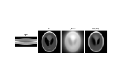
The Radon transform is the integral transform which takes a square image \(x\) defined on the plane to a function \(y=\forw{x}\) defined on the (two-dimensional) space of lines in the plane, whose value at a particular line is equal to the line integral of the function over that line.
Note
The pseudo-inverse is computed using the filtered back-projection algorithm with a Ramp filter. This is not the exact linear pseudo-inverse of the Radon transform, but it is a good approximation which is robust to noise.
Note
The measurements are not normalized by the image size, thus the norm of the operator depends on the image size.
Note
This operator only handles 2D images. For more advanced use-cases, see the
deepinv.physics.TomographyWithAstraoperator which handles 2D and 3D geometries.Warning
The adjoint operator has small numerical errors due to interpolation. Set
adjoint_via_backprop=Trueif you want to use the exact adjoint (computed via autograd).Warning
By default,
normalizeis set toTrueif not specified. Initializing the operator without specifying the normalization behavior will issue a warning. Note that normalizing the operator affects the reconstruction dynamics, which may not always be suitable for real-world applications.- Parameters:
angles (int, torch.Tensor) – These are the tomography angles. If the type is
int, the angles are sampled uniformly between 0 and 360 degrees. If the type istorch.Tensor, the angles are the ones provided (e.g.,torch.linspace(0, 180, steps=10)).img_width (int) – width/height of the square image input.
circle (bool) – If
Trueboth forward and backward projection will be restricted to pixels inside a circle inscribed in the square image.parallel_computation (bool) – if
True, all projections are performed in parallel. Requires more memory but is faster on GPUs.adjoint_via_backprop (bool) – if
True, the adjoint will be computed viadeepinv.physics.adjoint_function(). Otherwise the inverse Radon transform is used. The inverse Radon transform is computationally cheaper (particularly in memory), but has a small adjoint mismatch. The backprop adjoint is the exact adjoint, but might break random seeds since it backpropagates throughtorch.nn.functional.grid_sample(), see the note here.fbp_interpolate_boundary (bool) – the
filtered back-projectionusually contains streaking artifacts on the boundary due to padding. Forfbp_interpolate_boundary=Truethese artifacts are corrected by cutting off the outer two pixels of the FBP and recovering them by interpolating the remaining image. This option only makes sense ifcircleis set toFalse. Hence it will be ignored ifcircleis True.normalize (bool) – If
TrueAandA_adjointare normalized so that the operator has unit norm. (default:True)fan_beam (bool) – If
True, use fan beam geometry, ifFalseuse parallel beamfan_parameters (dict[str, int | float]) –
Only used if fan_beam is
True. Contains the parameters defining the scanning geometry. The dict should contain the keys:”pixel_spacing” defining the distance between two pixels in the image, default: 0.5 / (in_size)
”source_radius” distance between the x-ray source and the rotation axis (middle of the image), default: 57.5
”detector_radius” distance between the x-ray detector and the rotation axis (middle of the image), default: 57.5
”n_detector_pixels” number of pixels of the detector, default: 258
”detector_spacing” distance between two pixels on the detector, default: 0.077
The default values are adapted from the geometry in Khalil et al.[1]. where pixel spacing, source and detector radius and detector spacing are given in cm. Note that a to small value of n_detector_pixels*detector_spacing can lead to severe circular artifacts in any reconstruction.
device (str) – gpu or cpu.
- Examples:
Tomography operator with defined angles for 3x3 image:
>>> from deepinv.physics import Tomography
>>> seed = torch.manual_seed(0)  # Random seed for reproducibility
>>> x = torch.randn(1, 1, 4, 4)  # Define random 4x4 image
>>> angles = torch.linspace(0, 45, steps=3)
>>> physics = Tomography(angles=angles, img_width=4, circle=True, normalize=False)
>>> physics(x)
tensor([[[[ 0.0000, -0.1791, -0.1719],
          [-0.5713, -0.4521, -0.5177],
          [ 0.0340,  0.1448,  0.2334],
          [ 0.0000, -0.0448, -0.0430]]]])
Tomography operator with 3 uniformly sampled angles in [0, 360] for 3x3 image:
>>> from deepinv.physics import Tomography
>>> seed = torch.manual_seed(0)  # Random seed for reproducibility
>>> x = torch.randn(1, 1, 4, 4)  # Define random 4x4 image
>>> physics = Tomography(angles=3, img_width=4, circle=True, normalize=False)
>>> physics(x)
tensor([[[[ 0.0000, -0.1806,  0.0500],
          [-0.5713, -0.6076, -0.6815],
          [ 0.0340,  0.3175,  0.0167],
          [ 0.0000, -0.0452,  0.0989]]]])
- References:
- A(x, **kwargs)[source]#
Forward projection.
- Parameters:
x (torch.Tensor) – input of shape [B,C,H,W]
- Returns:
measurement of shape [B,C,A,N], with A the number of angular positions, and N the number of detector cells.
- Return type:
- A_adjoint(y, **kwargs)[source]#
Computes adjoint of the tomography operator.
Warning
The default adjoint operator has small numerical errors due to interpolation. Set
adjoint_via_backprop=Trueif you want to use the exact adjoint (computed via autograd).- Parameters:
y (torch.Tensor) – measurements of shape [B,C,A,N]
- Returns:
scaled back-projection of shape [B,C,H,W]
- Return type:
- A_dagger(y, fbp=False, **kwargs)[source]#
Computes the solution in \(x\) to \(y = Ax\) using a least squares solver. A faster approximation can be obtained by setting
fbp=True, which computes the filtered back-projection of the measurements.Warning
The filtered back-projection algorithm is not the exact linear pseudo-inverse of the Radon transform, but it is a good approximation that is robust to noise.
- Parameters:
y (torch.Tensor) – measurements of shape [B,C,A,N], with A the number of angular positions, and N the number of detector cells
- Returns:
filtered back-projection of shape [B,C,H,W]
- Return type:
- fbp(y, **kwargs)[source]#
Computes the filtered back-projection (FBP) of the measurements.
Tip
By default, the FBP reconstruction can display artifacts at the borders. Set
fbp_interpolate_boundary=Trueto remove them with padding.- Parameters:
y (torch.Tensor) – measurements of shape [B,C,A,N], with A the number of angular positions, and N the number of detector cells
- Returns:
filtered back-projection of shape [B,C,H,W]
- Return type:
Examples using Tomography:#
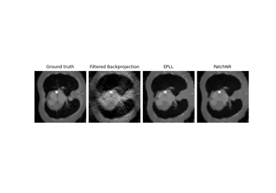
Patch priors for limited-angle computed tomography
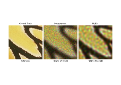
Poisson Inverse Problems with Maximum-Likelihood Expectation-Maximization (MLEM)

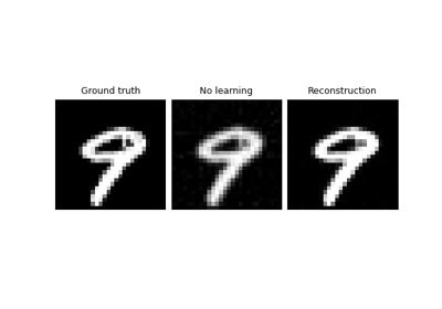
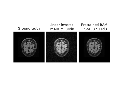
Self-supervised learning with measurement splitting