
Note
New to DeepInverse? Get started with the basics with the 5 minute quickstart tutorial..
Self-supervised learning with Equivariant Splitting#
Equivariant splitting consists in minimizing a self-supervised loss to train a reconstruction model using measurement data only [1].
It is based on the same assumption of invariance as equivariant imaging Self-supervised learning with Equivariant Imaging for MRI. Namely, the distribution of ground truth images is assumed to be invariant to certain transformations such as translations, rotations and flips.
Moreover, it is also based on splitting methods which separate measurements into inputs and targets \(y = [y_1^\top, y_2^\top]^\top\). The target measurements are not fed to the network and guide the network to learn to predict information that is not present in the input measurements.
The equivariant splitting loss combines the two approaches as:
where \(T_g\) denote a transformation and \(A T_g\) the associated virtual physics represented in the library by the class deepinv.physics.VirtualLinearPhysics. The loss itself is implemented in deepinv.loss.EquivariantSplittingLoss and this example shows how to use it to train a reconstruction model in a fully self-supervised way.
from pathlib import Path
import torch
from torch.utils.data import DataLoader
from torchvision import transforms
import os

import deepinv as dinv
Setup random seeds, paths and device#
# For reproducilibity
torch.manual_seed(0)
torch.cuda.manual_seed_all(0)
torch.backends.cudnn.deterministic = True

# Setup paths
BASE_DIR = Path(".")
DATA_DIR = BASE_DIR / "measurements"
CKPT_DIR = BASE_DIR / "ckpts"

# Select the device
device = dinv.utils.get_freer_gpu() if torch.cuda.is_available() else "cpu"
Selected GPU 0 with 1607.25 MiB free memory
Forward model#
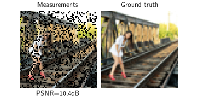
First, we define the forward model, here an inpainting problem with a fixed mask keeping 70% of pixels:
Create the imaging dataset#
Using the forward model and a base dataset, here deepinv.datasets.Urban100HR, we generate an imaging dataset that we further split into a 80 training samples, 19 evaluation samples and 1 test sample.
transform = transforms.Compose(
    [
        transforms.Resize(img_size),
        transforms.CenterCrop(img_size),
    ]
)

dataset = dinv.datasets.Urban100HR(
    root=dinv.utils.get_cache_home() / "datasets" / "Urban100",
    transform=transform,
    download=True,
)
train_dataset, eval_dataset, test_dataset = torch.utils.data.random_split(
    dataset, [80, 19, 1], generator=torch.Generator().manual_seed(0)
)

batch_size = 4
num_workers = 4 if torch.cuda.is_available() else 0

dataset_path = dinv.datasets.generate_dataset(
    train_dataset=train_dataset,
    val_dataset=eval_dataset,
    test_dataset=test_dataset,
    physics=physics,
    device=device,
    save_dir="Urban100",
    batch_size=batch_size,
    num_workers=num_workers,
)

train_dataset = dinv.datasets.HDF5Dataset(path=dataset_path, split="train")
eval_dataset = dinv.datasets.HDF5Dataset(path=dataset_path, split="val")
test_dataset = dinv.datasets.HDF5Dataset(path=dataset_path, split="test")

train_dataloader = DataLoader(
    train_dataset, batch_size=batch_size, num_workers=num_workers, shuffle=True
)
eval_dataloader = DataLoader(
    eval_dataset, batch_size=batch_size, num_workers=num_workers, shuffle=False
)
test_dataloader = DataLoader(
    test_dataset, batch_size=batch_size, num_workers=num_workers, shuffle=False
)
Dataset has been saved at Urban100/dinv_dataset0.h5
Visualizing the problem#
Create the base model#
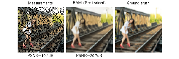
Here, we fine tune a pretrained deepinv.models.RAM model but any trainable reconstructor would do.
In order to track the improvements brought by fine-tuning the model, we also create a copy of the pre-trained model that will not be fine-tuned.
model = dinv.models.RAM(pretrained=True).to(device)
model_no_learning = dinv.models.RAM(pretrained=True).to(device)

model_no_learning.eval()
with torch.no_grad():
    x_pretrained = model_no_learning(y, physics)

psnr_pretrained = psnr_fn(x_pretrained, x).item()

dinv.utils.plot(
    [y, x_pretrained, x],
    ["Measurements", "RAM (Pre-trained)", "Ground truth"],
    subtitles=[f"PSNR={psnr_y:.1f}dB", f"PSNR={psnr_pretrained:.1f}dB", ""],
    fontsize=10,
)
Setup the equivariant splitting loss#
We create an instance of deepinv.loss.EquivariantSplittingLoss that implements the equivariant splitting loss.
The equivariant splitting loss requires the definition of a splitting scheme similarly to deepinv.loss.SplittingLoss. Here, we choose a pixel-wise Bernoulli splitting scheme with a split ratio of 0.9 using deepinv.physics.generator.BernoulliSplittingMaskGenerator.
Equivariant splitting requires choosing a set of transformations for which the forward operator is not equivariant. For inpainting, valid choices include shifts, rotations and reflections [1]. Here, we choose rotations and reflections.
Since the base model RAM is not already equivariant to these transformations, we use group averaging by passing in transform and eval_transform to the loss. Namely, we swap the base reconstructor \(\tilde{R}\) for the equivariant reconstructor defined by
which is estimated using a Monte Carlo sampling where a subset of transformations is used, typically a single one at training time and the full set at evaluation time. Internally, the input model is wrapped in an deepinv.models.EquivariantReconstructor when calling deepinv.loss.EquivariantSplittingLoss.adapt_model().
Note
The equivariant splitting loss consists in a prediction term and a consistency term. In the absence of noise, they are computed exactly using deepinv.loss.MCLoss. In the presence of noise, they can be estimated without bias using denoising losses such as deepinv.loss.R2RLoss and deepinv.loss.SureGaussianLoss.
# Splitting scheme
mask_generator = dinv.physics.generator.BernoulliSplittingMaskGenerator(
    img_size=(1, img_size, img_size),
    split_ratio=0.9,
    pixelwise=True,
    device=device,
)

# Underlying measurement comparison losses
consistency_loss = dinv.loss.MCLoss(metric=dinv.metric.MSE())
prediction_loss = dinv.loss.MCLoss(metric=dinv.metric.MSE())

# A random grid-preserving transformation
train_transform = dinv.transform.Rotate(
    n_trans=1, multiples=90, positive=True
) * dinv.transform.Reflect(n_trans=1, dim=[-1])
# All grid-preserving transformations
eval_transform = dinv.transform.Rotate(
    n_trans=4, multiples=90, positive=True
) * dinv.transform.Reflect(n_trans=2, dim=[-1])

es_loss = dinv.loss.EquivariantSplittingLoss(
    mask_generator=mask_generator,
    consistency_loss=consistency_loss,
    prediction_loss=prediction_loss,
    transform=train_transform,
    eval_transform=eval_transform,
    eval_n_samples=5,
)

# Wrap the model so it takes split measurements as input and apply Reynolds averaging
model = es_loss.adapt_model(model)
Train the model#
We fine-tune the pre-trained model using the equivariant splitting loss and early stopping with the validation loss as criterion. This makes the whole training fully self-supervised and usable when no ground truth image is available.
Note
We skip the training and directly load the cached checkpoint to avoid making the documentation longer to build but you can get the same results by running the training locally.
# Cached checkpoint after training to avoid doing the computation over and over
cached_checkpoint = (
    "https://huggingface.co/jscanvic/deepinv/resolve/main/ES/demo/ckp_best.pth.tar"
)

if cached_checkpoint is None:
    epochs = 20
    ckpt_pretrained = None
else:
    epochs = 0
    ckpt_pretrained = (
        dinv.utils.get_cache_home() / "examples" / "ES" / "ckp_best.pth.tar"
    )
    os.makedirs(ckpt_pretrained.parent, exist_ok=True)

    # Download if not found
    if not ckpt_pretrained.exists():
        torch.hub.download_url_to_file(cached_checkpoint, ckpt_pretrained)
    else:
        print(f"Checkpoint found at {ckpt_pretrained}, skipping download.")

    # Ignore RNG states from the checkpoint
    ckpt = torch.load(ckpt_pretrained, map_location=device, weights_only=True)
    state_dict = ckpt["state_dict"]
    current_state_dict = model.state_dict()
    for key in list(state_dict.keys()):
        if "initial_random_state" in key:
            state_dict[key] = current_state_dict[key]
    torch.save(ckpt, ckpt_pretrained)

trainer = dinv.Trainer(
    model,
    physics=physics,
    epochs=epochs,
    ckpt_pretrained=ckpt_pretrained,
    ckp_interval=epochs,
    scheduler=None,
    losses=[es_loss],
    optimizer=torch.optim.AdamW(model.parameters(), lr=5e-4, weight_decay=1e-8),
    train_dataloader=train_dataloader,
    eval_dataloader=eval_dataloader,
    metrics=[
        dinv.metric.PSNR()
    ],  # Supervised oracle metric for monitoring, not used for training and early stopping
    plot_images=False,
    device=device,
    verbose=True,
    show_progress_bar=False,
    no_learning_method=model_no_learning,
    compute_eval_losses=True,  # Compute eval losses
    early_stop=3,  # Patience parameter, stop if there is no improvement for multiple epochs
    early_stop_on_losses=True,  # Use the evaluation loss as a self-supervised stopping criterion
)

trainer.train()
if epochs > 0:
    trainer.load_best_model()
Checkpoint found at /local/jtachell/.cache/deepinv/examples/ES/ckp_best.pth.tar, skipping download.
/local/jtachell/deepinv/deepinv/deepinv/training/trainer.py:1337: UserWarning: non_blocking_transfers=True but DataLoader.pin_memory=False; set pin_memory=True to overlap host-device copies with compute.
  self.setup_train()
The model has 35618813 trainable parameters
Model, optimizer, epoch_start successfully loaded from checkpoint: /local/jtachell/.cache/deepinv/examples/ES/ckp_best.pth.tar
/local/jtachell/deepinv/deepinv/deepinv/training/trainer.py:548: UserWarning: No training will be done because epochs (0) <= loaded epoch_start (12) from checkpoint.
  warnings.warn(
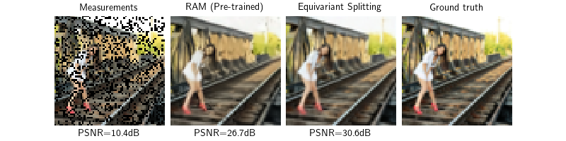
Evaluation of the trained model#
We can now evaluate the trained model on the test set using the PSNR metric.
We also compare it to the pre-trained model without fine-tuning to see the benefit of fine-tuning with equivariant splitting:
# Compute the performance metrics on the whole test set
trainer.compute_eval_losses = False
trainer.early_stop_on_losses = False
trainer.test(test_dataloader, metrics=dinv.metric.PSNR())

# Display the reconstructions for a single test sample
model.eval()

with torch.no_grad():
    x_hat = model(y, physics)

psnr = psnr_fn(x_hat, x).item()

dinv.utils.plot(
    [y, x_pretrained, x_hat, x],
    ["Measurements", "RAM (Pre-trained)", "Equivariant Splitting", "Ground truth"],
    subtitles=[
        f"PSNR={psnr_y:.1f}dB",
        f"PSNR={psnr_pretrained:.1f}dB",
        f"PSNR={psnr:.1f}dB",
        "",
    ],
    fontsize=10,
)
/local/jtachell/deepinv/deepinv/deepinv/training/trainer.py:1529: UserWarning: non_blocking_transfers=True but DataLoader.pin_memory=False; set pin_memory=True to overlap host-device copies with compute.
  self.setup_train(train=False)
Eval epoch 0: PSNR=26.542, PSNR no learning=23.163
Test results:
PSNR no learning: 23.163 +- 0.005
PSNR: 26.542 +- 0.005
- References:
Total running time of the script: (0 minutes 42.087 seconds)