Poisson-Gaussian Denoising with the Generalized Anscombe Transform

This example demonstrates how to denoise images corrupted by Poisson-Gaussian noise using the Generalized Anscombe Transform (GAT), which converts any Gaussian denoiser into a Poisson-Gaussian denoiser [1].

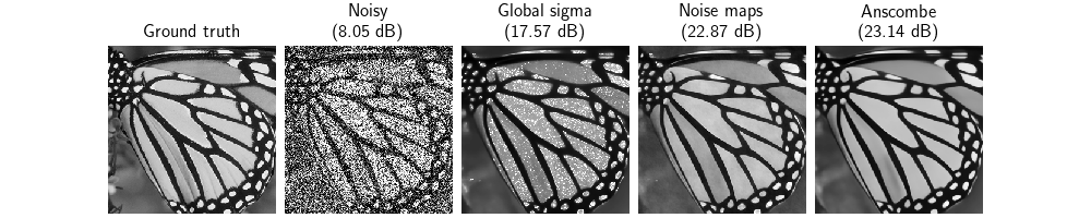
We compare three approaches on a butterfly image:

• DRUNet baseline – the pretrained DRUNet Gaussian denoiser applied directly to the noisy measurement, using a global noise-level heuristic.

• DRUNet with spatial noise maps – the pretrained DRUNet conditioned on spatial noise levels, which capture the variance of the Poisson-Gaussian noise at each pixel.

• Anscombe + DRUNet – the same DRUNet wrapped with AnscombeDenoiser, which first variance-stabilizes the heteroscedastic Poisson-Gaussian noise via the GAT.

Background

The Poisson-Gaussian noise model arises naturally in photon-counting imaging systems (fluorescence microscopy, astronomy, low-light photography), where the observed measurement \(y\) satisfies

\[y = \gamma \, z + \varepsilon, \qquad z \sim \mathcal{P}\!\left(\tfrac{x}{\gamma}\right),\; \varepsilon \sim \mathcal{N}(0, \sigma^2 I),\]

with photon gain \(\gamma > 0\) and read-out noise level \(\sigma \geq 0\).

The Generalized Anscombe Transform (GAT) stabilizes the variance of the Poisson-Gaussian noise to approximately \(\gamma^2\):

\[z = 2\sqrt{\gamma y + \tfrac{3}{8}\gamma^2 + \sigma^2}.\]

After applying the GAT the signal approximately follows a Gaussian distribution of standard deviation \(\gamma\), so any Gaussian denoiser trained at noise level \(\sigma_d=\gamma\). The inverse GAT maps back to the original domain. Setting \(u = z / \gamma\), it reads:

\[\hat{y} = \gamma \left( \frac{1}{4}u^2 + \frac{1}{4}\sqrt{\tfrac{3}{2}}\,u^{-1} - \frac{11}{8}u^{-2} + \frac{5}{8}\sqrt{\tfrac{3}{2}}\,u^{-3} - \frac{1}{8} - \frac{\sigma^2}{\gamma^2} \right), \qquad u = \frac{z}{\gamma}.\]

The full pipeline of AnscombeDenoiser reads:

\[\hat{x} = \mathrm{IGAT}\!\left(\denoisername\!\left(z,\; \sigma_d=\gamma\right)\right), \qquad z = \mathrm{GAT}(y).\]

Note

The formula varies slightly from the one proposed by Makitalo and Foi[1], as the library considers a normalized Poisson-Gaussian noise model, \(y = \gamma \mathcal{P}(x/\gamma) + \epsilon\), whereas the authors consider \(y = \gamma \mathcal{P}(x) + \epsilon\).

import torch
import deepinv as dinv
from deepinv.models import AnscombeDenoiser, DRUNet, PatchCovarianceNoiseEstimator
from deepinv.utils import load_example

device = dinv.utils.get_device()
torch.manual_seed(0)

Selected GPU 0 with 6664.25 MiB free memory

<torch._C.Generator object at 0x7f05ba810710>

Load a clean butterfly image

x = load_example("butterfly.png", device=device, grayscale=True)

Case 1: Poisson noise

In the pure Poisson model, the observed measurement \(y\) satisfies

\[y = \gamma \, z, \qquad z \sim \mathcal{P}\!\left(\tfrac{x}{\gamma}\right),\]

where \(\mathcal{P}(\lambda)\) denotes a Poisson random variable with rate \(\lambda\), \(x \geq 0\) is the clean image, and \(\gamma > 0\) is the photon gain. The variance of \(y\) is signal-dependent: \(\mathrm{Var}(y_i) = \gamma \, x_i\), making the noise heteroscedastic.

gain = 0.3  # photon gain gamma

physics_poisson = dinv.physics.Denoising(
    dinv.physics.PoissonNoise(gain=gain, clip_positive=True),
    device=device,
)

y_poisson = physics_poisson(x)

Verifying variance stabilization with the Anscombe transform

A key property of the GAT is that, after applying it to a Poisson-noisy image, the resulting signal is approximately Gaussian with a constant standard deviation equal to the gain \(\gamma\). We can verify this empirically by running a blind Gaussian noise-level estimator (PatchCovarianceNoiseEstimator) on the transformed image: the estimated \(\hat{\sigma}\) should be close to \(\gamma\).

with torch.no_grad():
    z = dinv.models.anscombe.generalized_anscombe_transform(
        y_poisson, gain=gain, sigma=0.0
    )
    sigma_est = PatchCovarianceNoiseEstimator()(z)
    print(
        f"Estimated noise level after Anscombe transform: {sigma_est.item():.4f}  (expected ≈ gain = {gain:.4f})"
    )

dinv.utils.plot([y_poisson, z], ["Noisy", "GAT(Noisy)"], rescale_mode="clip")

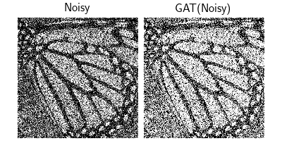
Estimated noise level after Anscombe transform: 0.2692  (expected ≈ gain = 0.3000)

Set up the Anscombe-wrapped DRUNet denoiser

DRUNet is a powerful Gaussian denoiser. We wrap it with AnscombeDenoiser to lift it to the Poisson-Gaussian domain. The GAT output has standard deviation approximately \(\gamma\), so the wrapper calls DRUNet at noise level \(\gamma\).

drunet = DRUNet(in_channels=1, out_channels=1, device=device)
anscombe_denoiser = AnscombeDenoiser(drunet)

Set up the plain DRUNet baselines (no Anscombe transform)

As baselines we apply DRUNet directly to the noisy measurement, using a noise-level heuristic derived from the Poisson-Gaussian variance. For Poisson-Gaussian noise, \(\mathrm{Var}(y_i) \approx \gamma x_i + \sigma^2\), so a reasonable single-number estimate of the noise standard deviation is:

\[\sigma_i = \sqrt{y_i \gamma + \frac{3}{8}\gamma^2 + \sigma^2},\]

For pure Poisson noise (\(\sigma = 0\)) this reduces to \(\sigma_i = \sqrt{(y_i + \frac{3}{8}\gamma) \cdot \gamma}\).

We can construct two baselines with this approximation

• Global average – the spatially averaged noise standard deviation \(\bar{\sigma} = \mathrm{mean}_i(\sigma_i)\) is applied uniformly to all pixels.

• Space-varying noise maps – each pixel gets its own noise level \(\sigma_i\), which is fed to DRUNet as a spatial noise map.

Denoise – pure Poisson scenario

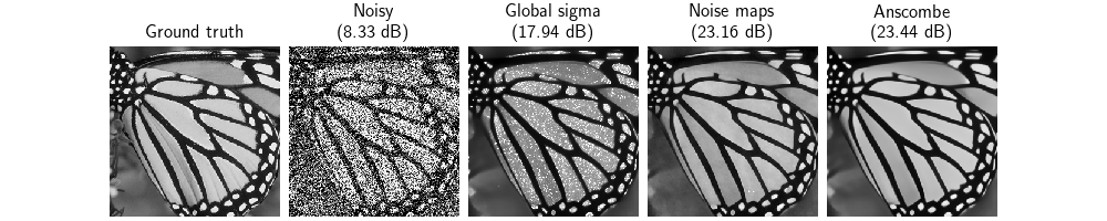
We first evaluate all methods on the pure Poisson case with \(\gamma=0.3\) and \(\sigma=0\)

with torch.no_grad():
    # Anscombe + DRUNet
    x_hat_anscombe_poisson = anscombe_denoiser(y_poisson, gain=gain, sigma=1e-6)

    # Plain DRUNet with space-varying approximate noise maps
    sigma_approx_poisson = ((3 / 8 * gain + y_poisson) * gain).clamp(min=1e-6) ** 0.5
    x_hat_drunet_poisson = drunet(y_poisson, sigma_approx_poisson)

    # Plain DRUNet with global (spatially averaged) noise level
    sigma_global_poisson = sigma_approx_poisson.mean() * torch.ones_like(
        sigma_approx_poisson
    )
    x_hat_drunet_global_poisson = drunet(y_poisson, sigma_global_poisson)


psnr = dinv.metric.PSNR()

# compute PSNR metrics
psnr_noisy_poisson = psnr(y_poisson, x).item()
psnr_anscombe_poisson = psnr(x_hat_anscombe_poisson, x).item()
psnr_drunet_poisson = psnr(x_hat_drunet_poisson, x).item()
psnr_drunet_global_poisson = psnr(x_hat_drunet_global_poisson, x).item()

dinv.utils.plot(
    [
        x,
        y_poisson,
        x_hat_drunet_global_poisson,
        x_hat_drunet_poisson,
        x_hat_anscombe_poisson,
    ],
    titles=[
        "Ground truth",
        f"Noisy\n({psnr_noisy_poisson:.2f} dB)",
        f"Global sigma\n({psnr_drunet_global_poisson:.2f} dB)",
        f"Noise maps\n({psnr_drunet_poisson:.2f} dB)",
        f"Anscombe\n({psnr_anscombe_poisson:.2f} dB)",
    ],
    rescale_mode="clip",
)

Case 2: Mixed Poisson-Gaussian noise

Secondly, we evaluate all methods on the pure Poisson case with \(\gamma=0.3\) and \(\sigma=0.1\)

sigma_pg = 0.1  # Gaussian read-out noise sigma

physics_pg = dinv.physics.Denoising(
    dinv.physics.PoissonGaussianNoise(gain=gain, sigma=sigma_pg, clip_positive=True),
    device=device,
)
y_pg = physics_pg(x)


with torch.no_grad():
    # Anscombe + DRUNet
    x_hat_anscombe_pg = anscombe_denoiser(y_pg, gain=gain, sigma=sigma_pg)

    # Plain DRUNet with space-varying approximate noise maps
    sigma_approx_maps_pg = ((gain * 3 / 8 + y_pg) * gain + sigma_pg**2).clamp(
        min=1e-6
    ) ** 0.5
    x_hat_drunet_pg = drunet(y_pg, sigma_approx_maps_pg)

    # Plain DRUNet with global (spatially averaged) noise level
    sigma_global_pg = sigma_approx_maps_pg.mean() * torch.ones_like(
        sigma_approx_maps_pg
    )
    x_hat_drunet_global_pg = drunet(y_pg, sigma_global_pg)


# compute PSNR metrics
psnr_noisy_pg = psnr(y_pg, x).item()
psnr_anscombe_pg = psnr(x_hat_anscombe_pg, x).item()
psnr_drunet_pg = psnr(x_hat_drunet_pg, x).item()
psnr_drunet_global_pg = psnr(x_hat_drunet_global_pg, x).item()

dinv.utils.plot(
    [x, y_pg, x_hat_drunet_global_pg, x_hat_drunet_pg, x_hat_anscombe_pg],
    titles=[
        "Ground truth",
        f"Noisy\n({psnr_noisy_pg:.2f} dB)",
        f"Global sigma\n({psnr_drunet_global_pg:.2f} dB)",
        f"Noise maps\n({psnr_drunet_pg:.2f} dB)",
        f"Anscombe\n({psnr_anscombe_pg:.2f} dB)",
    ],
    rescale_mode="clip",
)

Conclusion

All three DRUNet variants successfully suppress the Poisson-Gaussian noise.

• DRUNet with global sigma – uses a single spatially-averaged noise level This is the simplest baseline; it treats the noise as spatially uniform.

• DRUNet with noise maps – feeds a per-pixel noise-level map to DRUNet, providing spatial heteroscedasticity information but still operating in the original domain.

• AnscombeDenoiser is a zero-cost upgrade: wrap any off-the-shelf Gaussian denoiser to handle Poisson-Gaussian noise without re-training, by properly stabilizing the heteroscedastic Poisson variance via the GAT before denoising.

References:

[1] (1,2)

Markku Makitalo and Alessandro Foi. Optimal inversion of the generalized anscombe transformation for poisson-gaussian noise. IEEE transactions on image processing, 22(1):91–103, 2012.