Poisson Inverse Problems with Maximum-Likelihood Expectation-Maximization (MLEM)

This example demonstrates how to solve Poisson inverse problems using the Maximum-Likelihood Expectation-Maximization (MLEM) algorithm Shepp and Vardi[1], also known as the Richardson-Lucy algorithm in the deconvolution setting Richardson[2], Lucy[3].

The Poisson observation model is:

\[y \sim \mathcal{P}\!\left(\frac{Ax}{\gamma}\right)\]

where \(A\) is a linear forward operator, \(x \geq 0\) is the image to recover, \(\gamma > 0\) is the gain parameter, and \(\mathcal{P}\) denotes the Poisson distribution.

The MLEM algorithm solves the associated maximum-likelihood problem:

\[\underset{x \geq 0}{\operatorname{min}} \,\, \sum_i \left((Ax)_i - y_i \log((Ax)_i)\right)\]

using the following iterative update rule:

\[x^{k+1} = \frac{x^k}{A^\top \mathbf{1}} \odot A^\top\!\left(\frac{y}{Ax^k}\right)\]

where \(\odot\) denotes element-wise multiplication and the division is also element-wise. The MLEM algorithm is widely used in emission tomography such as Positron Emission Tomography (PET) and Single Photon Emission Computed Tomography (SPECT), where the Poisson noise model is a natural fit.

We show three scenarios of increasing complexity:

1. Deblurring with MLEM (no prior)

2. Deblurring with MLEM and Total-Variation (TV) prior

3. 2D Computed Tomography (CT) with MLEM and TV prior

import torch
import deepinv as dinv
from pathlib import Path
from torchvision import transforms

from deepinv.utils.demo import load_dataset, load_example
from deepinv.utils.plotting import plot, plot_curves

Setup

Set paths, device and random seed for reproducibility.

BASE_DIR = Path(".")
RESULTS_DIR = BASE_DIR / "results"

torch.manual_seed(0)
device = dinv.utils.get_freer_gpu() if torch.cuda.is_available() else "cpu"

We use a single image from the Set3C dataset.

img_size = 128 if torch.cuda.is_available() else 64
val_transform = transforms.Compose(
    [transforms.CenterCrop(img_size), transforms.ToTensor()]
)
dataset = load_dataset("set3c", transform=val_transform)
x = dataset[0].unsqueeze(0).to(device)  # ground-truth image

Deblurring with MLEM without prior

We create a Gaussian blur operator with Poisson noise. The MLEM/Richardson-Lucy algorithm is a standard approach for Poisson deconvolution without any prior.

# Define the blur kernel
n_channels = 3
filter_torch = dinv.physics.blur.gaussian_blur(sigma=(2, 2))

gain = 1 / 100
physics_blur = dinv.physics.BlurFFT(
    img_size=(n_channels, img_size, img_size),
    filter=filter_torch,
    device=device,
    noise_model=dinv.physics.PoissonNoise(
        gain=gain, normalize=True, clip_positive=True
    ),
)

# Generate noisy blurred observation
y_blur = physics_blur(x)

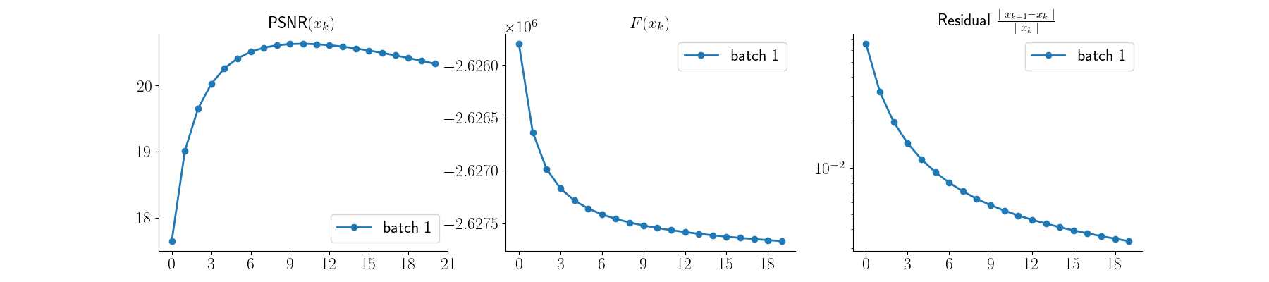
The deepinv.optim.MLEM class wraps the MLEM iterations. Without a prior, and in the case of deconvolution, this is equivalent to the classic Richardson-Lucy algorithm. Note that without prior, the algorithm will create artifacts when noise is present in the observation.

data_fidelity = dinv.optim.PoissonLikelihood(gain=gain)

model_no_prior = dinv.optim.MLEM(
    data_fidelity=data_fidelity,
    prior=None,
    max_iter=20,
    early_stop=True,
    thres_conv=1e-6,
    crit_conv="residual",
    verbose=True,
)

x_mlem, metrics_mlem = model_no_prior(
    y_blur, physics_blur, x_gt=x, compute_metrics=True
)

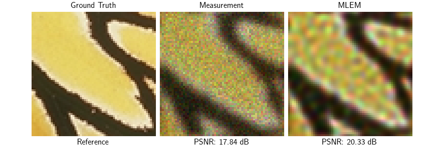
Visualize results and PSNR values along with convergence curves

psnr_input = dinv.metric.PSNR()(x, y_blur)
psnr_mlem = dinv.metric.PSNR()(x, x_mlem)

plot(
    {
        "Ground Truth": x,
        "Measurement": y_blur,
        "MLEM": x_mlem,
    },
    subtitles=[
        "Reference",
        f"PSNR: {psnr_input.item():.2f} dB",
        f"PSNR: {psnr_mlem.item():.2f} dB",
    ],
    figsize=(9, 3),
)

plot_curves(metrics_mlem)

• 
• 

Deblurring with MLEM + TV prior

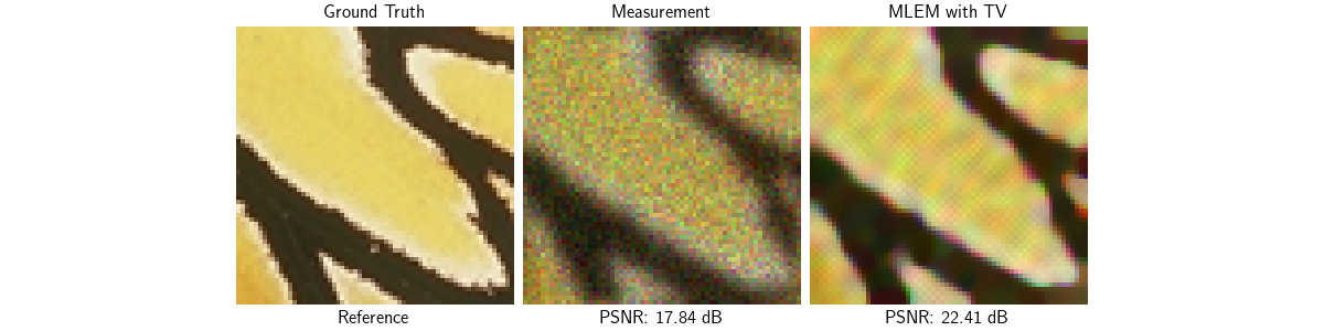
As we saw, MLEM tends to amplify noise when no prior information is used. Adding a Total-Variation (TV) prior solves this issue while favoring piecewise constant solutions. There are several ways of modifying MLEM for regularized objectives: here we use the most straightforward approach called One-Step-Late (OSL) [4] which simply adds the gradient of the prior to the denominator of the MLEM update:

\[x^{k+1} = \frac{x^k}{A^\top \mathbf{1} + \lambda \nabla \regname(x^k)} \odot A^\top\!\left(\frac{y}{Ax^k}\right)\]

For non-smooth regularizations, the penalized MLEM update becomes:

\[x^{k+1} = \frac{x^k}{A^\top \mathbf{1} + \lambda g^k} \odot A^\top\!\left(\frac{y}{Ax^k}\right), \quad g^k \in \partial \regname(x^k)\]

where \(\partial \regname(x^k)\) is the subdifferential of the regularization at \(x^k\). Any prior implementing the deepinv.optim.prior.Prior interface can be used in the deepinv.optim.MLEM class, and the proximal step is automatically computed when needed.

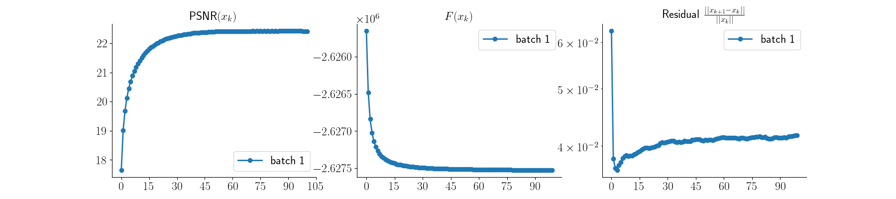
prior_tv = dinv.optim.prior.TVPrior(n_it_max=50)

model_tv = dinv.optim.MLEM(
    data_fidelity=data_fidelity,
    prior=prior_tv,
    lambda_reg=0.02,
    max_iter=100,
    early_stop=True,
    thres_conv=1e-6,
    crit_conv="residual",
    verbose=True,
)

x_mlem_tv, metrics_mlem_tv = model_tv(
    y_blur, physics_blur, x_gt=x, compute_metrics=True
)

Visualize results — MLEM + TV

psnr_mlem_tv = dinv.metric.PSNR()(x, x_mlem_tv)

plot(
    {
        "Ground Truth": x,
        "Measurement": y_blur,
        # "MLEM": x_mlem,
        "MLEM with TV": x_mlem_tv,
    },
    subtitles=[
        "Reference",
        f"PSNR: {psnr_input.item():.2f} dB",
        # f"PSNR: {psnr_mlem.item():.2f} dB",
        f"PSNR: {psnr_mlem_tv.item():.2f} dB",
    ],
    figsize=(12, 3),
)

plot_curves(metrics_mlem_tv)

• 
• 

Computed Tomography with MLEM + TV + custom metrics

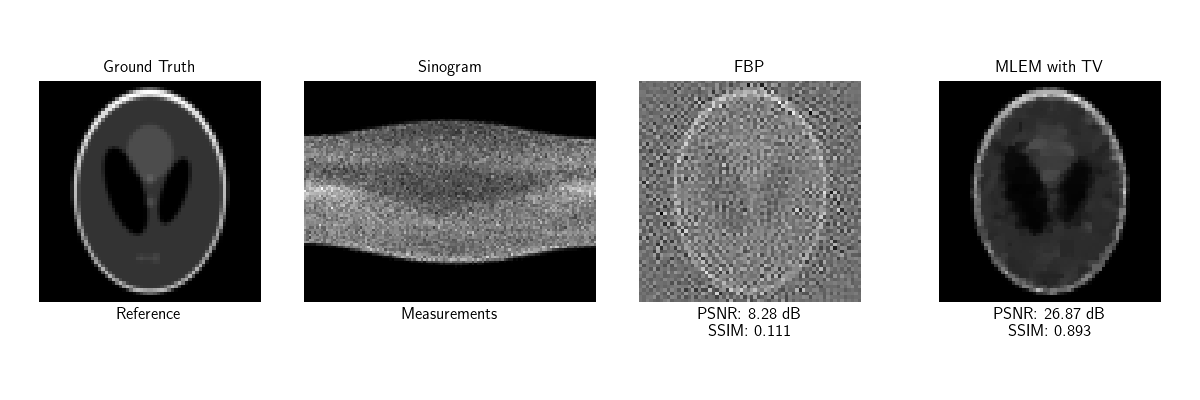
In emission tomography (PET/SPECT), the forward model is a Radon transform with Poisson statistics. Here we take the simple Shepp-Logan phantom as ground truth and use MLEM with TV prior to reconstruct it from its noisy sinogram.

# Load a grayscale image
val_transform_gray = transforms.Compose(
    [
        transforms.CenterCrop(img_size),
        transforms.Grayscale(num_output_channels=1),
        transforms.ToTensor(),
    ]
)
x_ct = load_example(
    "SheppLogan.png",
    img_size=img_size,
    grayscale=True,
    resize_mode="resize",
    device=device,
)

Set up Tomography physics We define a parallel-beam tomography operator with 120 projection angles uniformly distributed between 0° and 180°, and Poisson noise.

num_angles = 120
gain_ct = 1 / 300

physics_ct = dinv.physics.Tomography(
    img_width=img_size,
    angles=num_angles,
    device=device,
    noise_model=dinv.physics.PoissonNoise(
        gain=gain_ct, normalize=True, clip_positive=True
    ),
)

# Generate sinogram
y_ct = physics_ct(x_ct)
# Filtered back-projection as a simple baseline
x_fbp = physics_ct.A_dagger(y_ct)

/local/jtachell/deepinv/deepinv/deepinv/physics/tomography.py:187: UserWarning: The default value of `normalize` is not specified and will be automatically set to `True`. Set `normalize` explicitly to `True` or `False` to avoid this warning.
  warn(
/local/jtachell/deepinv/deepinv/deepinv/physics/forward.py:487: UserWarning: Following torch.nn.Module's design, the 'device' attribute is deprecated and will be removed in a future version. To move the module's buffers/parameters to a different device, use the `to()` method.
  warnings.warn(

Run MLEM + TV on the CT problem

data_fidelity_ct = dinv.optim.PoissonLikelihood(gain=gain_ct)
prior_tv_ct = dinv.optim.prior.TVPrior(n_it_max=50)

model_ct = dinv.optim.MLEM(
    data_fidelity=data_fidelity_ct,
    prior=prior_tv_ct,
    lambda_reg=1e-2,
    max_iter=50,
    early_stop=True,
    thres_conv=1e-6,
    crit_conv="residual",
    verbose=True,
)

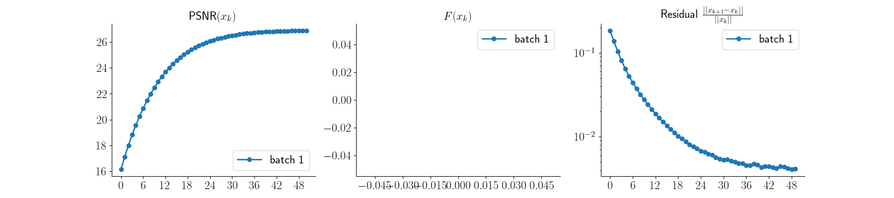
x_ct_recon, metrics_ct = model_ct(y_ct, physics_ct, x_gt=x_ct, compute_metrics=True)

Visualize CT results and plot convergence curves

psnr_fbp = dinv.metric.PSNR()(x_ct, x_fbp)
psnr_ct = dinv.metric.PSNR()(x_ct, x_ct_recon)
ssim_fbp = dinv.metric.SSIM()(x_ct, x_fbp)
ssim_ct = dinv.metric.SSIM()(x_ct, x_ct_recon)

plot(
    {
        "Ground Truth": x_ct,
        "Sinogram": y_ct,
        "FBP": x_fbp,
        "MLEM with TV": x_ct_recon,
    },
    subtitles=[
        "Reference",
        "Measurements",
        f"PSNR: {psnr_fbp.item():.2f} dB\nSSIM: {ssim_fbp.item():.3f}",
        f"PSNR: {psnr_ct.item():.2f} dB\nSSIM: {ssim_ct.item():.3f}",
    ],
    figsize=(12, 4),
)

plot_curves(metrics_ct)

• 
• 

References:

[1]

Lawrence A Shepp and Yehuda Vardi. Maximum likelihood reconstruction for emission tomography. IEEE Transactions on Medical Imaging, 1(2):113–122, 1982.

[2]

William Hadley Richardson. Bayesian-based iterative method of image restoration. Journal of the Optical Society of America, 62(1):55, 1972. doi:10.1364/JOSA.62.000055.

[3]

L. B. Lucy. An iterative technique for the rectification of observed distributions. The Astronomical Journal, 79:745, 1974. doi:10.1086/111605.

[4]

Peter J. Green. On Use of the Em Algorithm for Penalized Likelihood Estimation. Journal of the Royal Statistical Society: Series B (Methodological), 52(3):443–452, 1990. doi:10.1111/j.2517-6161.1990.tb01798.x.