
TomographyWithAstra#
- class deepinv.physics.TomographyWithAstra(img_size, angles=180, n_detector_pixels=None, angular_range=(0, 180), detector_spacing=1.0, pixel_spacing=1.0, bounding_box=None, geometry_type='parallel', geometry_parameters=MappingProxyType({'source_radius': 80.0, 'detector_radius': 20.0}), geometry_vectors=None, normalize=None, device=torch.device('cuda'), **kwargs)[source]#
Bases:
LinearPhysicsComputed Tomography operator with astra-toolbox backend. It is more memory efficient than the
deepinv.physics.Tomographyoperator and support 3D geometries. See documentation ofdeepinv.physics.functional.XrayTransformfor more information on theastrawrapper.Mathematically, it is described as a ray transform \(A\) which linearly integrates an object \(x\) along straight lines
\[y = \forw{x}\]where \(y\) is the set of line integrals, called sinogram in 2D, or radiographs in 3D. An object is typically scanned using a surrounding circular trajectory. Given different acquisition systems, the lines along which the integrals are computed follow different geometries:
- parallel. (2D and 3D)
Per view, all rays intersecting the object are parallel. In 2D, all rays live on the same plane, perpendicular to the axis of rotation.
- fanbeam. (2D)
Per view, all rays come from a single source and intersect the object at a certain angle. The detector consists of a 1d line of cells. Similar to the 2D “parallel”, all rays live on the same plane, perpendicular to the axis of rotation.
- conebeam. (3D)
Per view, all rays come from a single source. The detector consists of a 2D grid of cells. Apart from the central plane, the set of rays coming onto a line of cells live on a tilted plane.
Note
The pseudo-inverse is computed using the filtered back-projection algorithm with a Ramp filter, and its equivalent for conebeam 3D, the Feldkamp-Davis-Kress algorithm. This is not the exact linear pseudo-inverse of the Ray Transform, but it is a good approximation which is robust to noise.
Note
In the default configuration, reconstruction cells and detector cells are set to have isotropic unit lengths. The geometry is set to 2D parallel and matches the default configuration of the
deepinv.physics.Tomographyoperator withcircle=False.Warning
By default,
normalizeis set toTrueif not specified. Initializing the operator without specifying the normalization behavior will issue a warning. Note that normalizing the operator affects the reconstruction dynamics, which may not always be suitable for real-world applications.Warning
Due to computational efficiency reasons, the projector and backprojector implemented in
astraare not matched. The projector is typically ray-driven, while the backprojector is pixel-driven. The adjoint of the forward Ray Transform is approximated by rescaling the backprojector.Warning
The
deepinv.physics.functional.XrayTransformused indeepinv.physics.TomographyWithAstrasequentially processes batch elements, which can make the 2D parallel beam operator significantly slower than its native torch counterpart withdeepinv.physics.Tomography(though still more memory-efficient).- Parameters:
img_size (tuple[int, ...]) – Shape of the object grid, either a 2 or 3-element tuple, for respectively 2D or 3D.
angles (int) – Number of angular positions sampled uniformly in
angular_rangeor a Tensor containing angular positions in degrees. (default: 180)n_detector_pixels (int | tuple[int, ...], None) – In 2D, specify an integer for a single line of detector cells. In 3D, specify a 2-element tuple for (row,col) shape of the detector. (default: None)
angular_range (tuple[float, float]) – Angular range, defaults to
(0, 180).detector_spacing (float | tuple[float, float]) – In 2D the width of a detector cell. In 3D a 2-element tuple specifying the (vertical, horizontal) dimensions of a detector cell. (default: 1.0)
pixel_spacing (float | tuple[float, ...]) – In 2D, the (x,y) dimensions of a pixel in the reconstructed image. In 3D, the (x,y,z) dimensions of a voxel. Scalar value is interpreted as the same dimension along all axes (default: 1.0)
bounding_box (tuple[float, ...], None) – Axis-aligned bounding-box of the reconstruction area [min_x, max_x, min_y, max_y, …]. Optional argument, if specified, overrides argument
object_spacing. (default: None)geometry_type (str) – The type of geometry among
'parallel','fanbeam'in 2D and'parallel'and'conebeam'in 3D. (default:'parallel')geometry_parameters (dict[str, float]) –
Contains extra parameters specific to certain geometries. When
geometry_type='fanbeam'or'conebeam', the dictionary should contains the keys"source_radius": the distance between the x-ray source and the rotation axis, denoted \(D_{s0}\), (default: 80.),"detector_radius": the distance between the x-ray detector and the rotation axis, denoted \(D_{0d}\). (default: 20.)
geometry_vectors (torch.Tensor, None) –
Alternative way to describe a 3D geometry. It is a torch.Tensor of shape [num_angles, 12], where for each angular position of index
ithe row consists of a vector of size (12,) with(sx, sy, sz): the position of the source,(dx, dy, dz): the center of the detector,(ux, uy, uz): the horizontal unit vector of the detector,(vx, vy, vz): the vertical unit vector of the detector.
When specified,
geometry_vectorsoverridesdetector_spacing,anglesandgeometry_parameters. It is particularly useful to build the geometry for the Walnut-CBCT dataset, where the acquisition parameters are provided via such vectors.normalize (bool) – If
TrueA()andA_adjoint()are normalized so that the operator has unit norm. (default:True)device (torch.device | str) – The operator only supports CUDA computation. (default:
torch.device('cuda'))
- Examples:
Tomography operator with a 2D
'fanbeam'geometry, 10 uniformly sampled angles in[0, 360], a detector line of 5 cells with length 2., a source-radius of 20.0 and a detector_radius of 20.0 for 5x5 image:>>> import torch >>> if torch.cuda.is_available(): ... from deepinv.physics import TomographyWithAstra ... x = torch.randn(1, 1, 5, 5, device='cuda') # Define random 5x5 image ... physics = TomographyWithAstra( ... img_size=(5,5), ... angles=10, ... angular_range=(0, 360), ... n_detector_pixels=5, ... detector_spacing=2.0, ... geometry_type='fanbeam', ... geometry_parameters={ ... 'source_radius': 20., ... 'detector_radius': 20. ... }, ... normalize=False ... ) ... sinogram = physics(x) ... print(sinogram.shape) ... else: ... print(torch.Size([1, 1, 10, 5])) torch.Size([1, 1, 10, 5])
Tomography operator with a 3D
'conebeam'geometry, 10 uniformly sampled angles in[0, 360], a detector grid of 5x5 cells of size (2.,2.), a source-radius of 20.0 and a detector_radius of 20.0 for a 5x5x5 volume:>>> if torch.cuda.is_available(): ... x = torch.randn(1, 1, 5, 5, 5, device='cuda') # Define random 5x5x5 volume ... angles = torch.linspace(0, 360, steps=4)[:-1] ... physics = TomographyWithAstra( ... img_size=(5,5,5), ... angles = angles, ... n_detector_pixels=(5,5), ... pixel_spacing=(1.0,1.0,1.0), ... detector_spacing=(2.0,2.0), ... geometry_type='conebeam', ... geometry_parameters={ ... 'source_radius': 20., ... 'detector_radius': 20. ... }, ... normalize=False ... ) ... sinogram = physics(x) ... print(sinogram.shape) ... else: ... print(torch.Size([1, 1, 5, 3, 5])) torch.Size([1, 1, 5, 3, 5])
Note
This class requires the
astra-toolboxpackage to be installed. Install withpip install astra-toolbox.- A(x, **kwargs)[source]#
Forward projection.
In 2D, the output is a sinogram of shape [B,C,A,N], with A the number of angular positions, and N the number of detector cells. In 3D, the output is a stack of sinograms of shape [B,C,V,A,N], with A the number of angular positions, and (V,N) the shape of the 2D detector grid, where V is the number of rows of the detector and N the number of columns. :param torch.Tensor x: input of shape [B,C,…,H,W] :return: projection of shape [B,C,…,A,N]
- A_adjoint(y, **kwargs)[source]#
Approximation of the adjoint.
In 2D, expected input is a sinogram of shape [B,C,A,N], with A the number of angular positions, and N the number of detector cells. In 3D, expected input is a stack of sinograms of shape [B,C,V,A,N], with A the number of angular positions, and (V,N) the shape of the 2D detector grid, where V is the number of rows of the detector and N the number of columns.
- Parameters:
y (torch.Tensor) – input of shape [B,C,…,A,N]
- Returns:
scaled back-projection of shape [B,C,…,H,W]
- Return type:
- A_dagger(y, fbp=False, **kwargs)[source]#
Computes the solution in \(x\) to \(y = Ax\) using a least squares solver. A faster approximation can be obtained by setting
fbp=True, which computes the filtered back-projection of the measurements, or the Feldkamp-Davis-Kress algorithm (FDK) in cone-beam 3D.Warning
The filtered back-projection algorithm is not the exact linear pseudo-inverse of the Radon transform, but it is a good approximation that is robust to noise.
- Parameters:
y (torch.Tensor) – input of shape [B,C,…,A,N]
- Returns:
filtered back-projection of shape [B,C,…,H,W]
- Return type:
- fbp_weighting(sinogram)[source]#
Scales the computation by the inverse number of views and object-to-detector cell ratio.
In conebeam 3D, compute FDK weights to correct inflated distances due to tilted rays. Given coordinate \((x,y)\) of a detector cell, the corresponding weight is \(\omega(x,y) = \frac{D_{s0}}{\sqrt{D_{sd}^2 + x^2 + y^2}}\).
- Parameters:
sinogram (torch.Tensor) – Sinogram of shape [B,C,…,A,N].
- Returns:
Weighted sinogram.
- Return type:
Examples using TomographyWithAstra:#
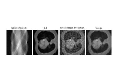
Low-dose CT with ASTRA backend and Total-Variation (TV) prior