ItohFidelity#
- class deepinv.optim.ItohFidelity(sigma=1.0, threshold=1.0)[source]#
Bases:
L2Itoh data-fidelity term for spatial unwrapping problems.
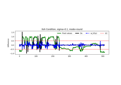
This class implements a data-fidelity term based on the \(\ell_2\) norm, but applied to the spatial finite differences of the variable and the wrapped differences of the data. This is based on the Itoh condition for phase unwrapping [1]. It is designed to be used in conjunction with the
deepinv.physics.SpatialUnwrappingclass for spatial unwrapping tasks.The data-fidelity term is defined as:
\[f(x,y) = \frac{1}{2\sigma^2} \| D x - w_{t}(Dy) \|^2\]where \(D\) denotes the spatial finite differences operator, \(w_t\) denotes the wrapping operator, and \(\sigma\) denotes the noise level.
- Parameters:
- Example:
>>> import torch
>>> from deepinv.physics.spatial_unwrapping import SpatialUnwrapping
>>> from deepinv.optim.data_fidelity import ItohFidelity
>>> x = torch.ones(1, 1, 3, 3)
>>> y = x
>>> physics = SpatialUnwrapping(threshold=1.0, mode="round")
>>> fidelity = ItohFidelity(sigma=1.0)
>>> f = fidelity(x, y, physics)
>>> print(f)
tensor([0.])
- References:
- D(x, **kwargs)[source]#
Apply spatial finite differences to the input tensor.
Computes the horizontal and vertical finite differences of the input tensor
xusing first-order differences along the last two spatial dimensions. The result is a tensor containing both the horizontal and vertical gradients stacked along a new dimension.- Parameters:
x (torch.Tensor) – Input tensor of shape (…, H, W), where H and W are spatial dimensions.
- Returns:
(
torch.Tensor) of shape (…, H, W, 2), where the last dimension contains the horizontal and vertical finite differences, respectively.- Return type:
- D_adjoint(x, **kwargs)[source]#
Applies the adjoint (transpose) of the spatial finite difference operator to the input tensor.
This function computes the adjoint operation corresponding to spatial finite differences, typically used in image processing and variational optimization problems. The input
xis expected to have its last dimension of size 2, representing the horizontal and vertical finite differences \((D_h x, D_v x)\).- Parameters:
x (torch.Tensor) – Input tensor of shape (…, 2), where the last dimension contains the horizontal and vertical finite differences.
- Returns:
(
torch.Tensor) The result of applying the adjoint finite difference operator, with the same shape as the input except for the last dimension (which is removed).- Return type:
- WD(x, **kwargs)[source]#
Applies spatial finite differences to the input and wraps the result.
This method computes the spatial finite differences of the input tensor \(x\) using the \(D\) operator, then applies modular rounding to the result. This is typically used in applications where periodic boundary conditions or phase wrapping are required.
- Parameters:
x (torch.Tensor) – Input tensor to which the spatial finite differences and wrapping are applied.
- Returns:
(
torch.Tensor) The wrapped finite differences of the input tensor.- Return type:
- fn(x, y, physics, *args, **kwargs)[source]#
Computes the data fidelity term \(\datafid{x}{y} = \distance{Dx}{w_{t}(Dy)}\).
- Parameters:
x (torch.Tensor) – Variable \(x\) at which the data fidelity is computed.
y (torch.Tensor) – Data \(y\).
physics (deepinv.physics.Physics) – physics model.
- Returns:
(
torch.Tensor) data fidelity \(\datafid{x}{y}\).
- grad(x, y, *args, **kwargs)[source]#
Calculates the gradient of the data fidelity term \(\datafidname\) at \(x\).
The gradient is computed using the chain rule:
\[\nabla_x \distance{Dx}{w_{t}(Dy)} = \left. \frac{\partial D}{\partial x} \right|_x^\top \nabla_u \distance{u}{w_{t}(Dy)},\]where \(\left. \frac{\partial D}{\partial x} \right|_x\) is the Jacobian of \(D\) at \(x\), and \(\nabla_u \distance{u}{w_{t}(Dy)}\) is computed using
grad_dwith \(u = Dx\). The multiplication is computed using theD_adjointmethod of the class.- Parameters:
x (torch.Tensor) – Variable \(x\) at which the gradient is computed.
y (torch.Tensor) – Data \(y\).
- Returns:
(
torch.Tensor) gradient \(\nabla_x \datafid{x}{y}\), computed in \(x\).- Return type:
- grad_d(u, y, *args, **kwargs)[source]#
Computes the gradient \(\nabla_u\distance{u}{w_{t}(Dy)}\), computed in \(u\).
Note that this is the gradient of \(\distancename\) and not \(\datafidname\). This function directly calls
deepinv.optim.Potential.grad()for the specific distance function \(\distancename\).- Parameters:
u (torch.Tensor) – Variable \(u\) at which the gradient is computed.
y (torch.Tensor) – Data \(y\) of the same dimension as \(u\).
- Returns:
(
torch.Tensor) gradient of \(d\) in \(u\), i.e. \(\nabla_u\distance{u}{w_{t}(Dy)}\).- Return type:
- prox(x, y, physics=None, *args, gamma=1.0, **kwargs)[source]#
Proximal operator of \(\gamma \datafid{x}{y}\)
Compute the proximal operator of the fidelity term \(\operatorname{prox}_{\gamma \datafidname}\), i.e.
\[\operatorname{prox}_{\gamma \datafidname} = \underset{u}{\text{argmin}} \frac{\gamma}{2\sigma^2}\|Du-w_{t}(Dy)\|_2^2+\frac{1}{2}\|u-x\|_2^2\]using the DCT-based closed-form solution of Ramirez et al.[2] as follows
\[\hat{x}_{i,j} = \texttt{DCT}^{-1}\left( \frac{\texttt{DCT}(D^{\top}w_t(Dy) + \frac{\rho}{2} z)_{i,j}} { \frac{\rho}{2} + 4 - (2\cos(\pi i / M) + 2\cos(\pi j / N))} \right)\]where \(D\) is the finite difference operator and \(\texttt{DCT}\) is the discrete cosine transform.
- Parameters:
x (torch.Tensor) – Variable \(x\) at which the proximity operator is computed.
y (torch.Tensor) – Data \(y\).
gamma (float) – stepsize of the proximity operator.
- Returns:
(
torch.Tensor) proximity operator \(\operatorname{prox}_{\gamma \datafidname}(x)\).- Return type:
- References:
- prox_d(u, y, *args, **kwargs)[source]#
Computes the proximity operator \(\operatorname{prox}_{\gamma\distance{\cdot}{w_{t}(Dy)}}(u)\), computed at \(u\).
Note that this is the proximity operator of \(\distancename\) and not \(\datafidname\). This function directly calls
deepinv.optim.Potential.prox()for the specific distance function \(\distancename\).- Parameters:
u (torch.Tensor) – Variable \(u\) at which the gradient is computed.
y (torch.Tensor) – Data \(y\) of the same dimension as \(u\).
- Returns:
(
torch.Tensor) gradient of \(d\) in \(u\), i.e. \(\nabla_u\distance{u}{w_{t}(Dy)}\).- Return type: